ARTÍCULOS – INGENIERÍAS

TEMPORAL DICTIONARY LEARNING FOR TIME-SERIES DECOMPOSITION

APRENDIZAJE DE DICCIONARIOS TEMPORALES PARA LA DESCOMPOSICIÓN DE SERIES DE TIEMPOS

Jens Bürger and Jorge Calvimontes

Institute for Computational Intelligence (ICI) ]]> Universidad Privada Boliviana
jensburger@upb.edu

(Recibido el 04 junio 2019, aceptado para publicación el 26 junio 2019)

ABSTRACT 

Dictionary Learning (DL) is a feature learning method that derives a finite collection of dictionary elements (atoms) from a given dataset. These atoms are small characteristic features representing recurring patterns within the data. A dictionary therefore is a compact representation of complex or large scale datasets. In this paper we investigate DL for temporal signal decomposition and reconstruction. Decomposition is a common method in time-series forecasting to separate a complex composite signal into different frequency components as to reduce forecasting complexity. By representing characteristic features, we consider dictionary elements to function as filters for the decomposition of temporal signals. Rather than simple filters with clearly defined frequency spectra, we hypothesize for dictionaries and the corresponding reconstructions to act as more complex filters. Training different dictionaries then permits to decompose the original signal into different components. This makes it a potential alternative to existing decomposition methods. We apply a known sparse DL algorithm to a wind speed dataset and investigate decomposition quality and filtering characteristics. Reconstruction accuracy serves as a proxy for evaluating the dictionary quality and a coherence analysis is performed to analyze how different dictionary configurations lead to different filtering characteristics. The results of the presented work demonstrate how learned features of different dictionaries represent transfer functions corresponding to frequency components found in the original data. Based on finite sets of atoms, dictionaries provide a deterministic mechanism to decompose a signal into various reconstructions and their respective remainders. These insights have direct application to the investigation and development of advanced signal decomposition and forecasting techniques.

Keywords: Dictionary Learning, SAILnet, Time-Series, Decomposition.

RESUMEN 

Dictionary Learning (DL) es un método de aprendizaje de características que deriva una colección finita de elementos del diccionario (átomos) de un conjunto de datos determinado. Estos átomos son pequeños rasgos característicos que representan patrones recurrentes dentro de los datos. Por lo tanto, un diccionario es una representación compacta de conjuntos de datos complejos o de gran escala. En este trabajo investigamos DL para la descomposición y reconstrucción de señales temporales. La descomposición es un método común en el pronóstico de series de tiempo para separar una señal compuesta compleja en diferentes componentes de frecuencia para reducir la complejidad del pronóstico. Al representar los rasgos característicos, consideramos que los elementos del diccionario funcionan como filtros para la descomposición de las señales temporales. En lugar de filtros simples con espectros de frecuencia claramente definidos, planteamos la hipótesis de que los diccionarios y las reconstrucciones correspondientes actúen como filtros más complejos. La capacitación de diferentes diccionarios permite luego descomponer la señal original en diferentes componentes. Esto lo convierte en una alternativa potencial a los métodos de descomposición existentes. Aplicamos un algoritmo de DL disperso conocido a un conjunto de datos de velocidad del viento e investigamos la calidad de descomposición y las características de filtrado. La precisión de la reconstrucción sirve como un proxy para evaluar la calidad del diccionario y se realiza un análisis de coherencia para analizar cómo diferentes configuraciones de diccionarios llevan a diferentes características de filtrado. Los resultados del trabajo presentado demuestran cómo las características aprendidas de diferentes diccionarios representan funciones de transferencia correspondientes a los componentes de frecuencia encontrados en los datos originales. Basados ​​en conjuntos finitos de átomos, los diccionarios proporcionan un mecanismo determinista para descomponer una señal en varias reconstrucciones y sus respectivos residuos. Estos conocimientos tienen una aplicación directa en la investigación y el desarrollo de técnicas avanzadas de descomposición de señales y pronóstico.

1. INTRODUCTION

Mammalian visual and auditory processing, located in the visual and auditory cortices, rely on a layered reconstruction of complex sensory information based on a finite set of simple features. In the primary visual cortex (V1) features such as edges are often represented by Gabor filters. Likely the most well-known example for such a layered sensory information processing structure is deep convolutional neural networks (deep learning) [1]. Another class of algorithms for feature learning is known as Dictionary Learning (DL) [2]. While deep learning is most commonly used as a supervised learning scheme for classification tasks, DL is a mostly unsupervised learning approach that aims to find a set of features permitting sparse representation of the data at hand. Such a sparse representation (or sparse code) allows reconstructing, with some degree of error ε, any complex signal with a linear combination of few features. Such a sparse representation of complex signals holds significant potential in signal decomposition where one wants to find a small set of signal components that describe underlying patterns and therefore permit separate analysis and processing of different types of patterns. Especially in time-series processing decomposition methods are standard tools in analysis and forecasting [3]. However, many decomposition methods are rather simplistic in relation to the signals they are trying to decompose. For example, STL decomposition (Seasonal and Trend decomposition using Loess) separates a signal into trend, seasonality and a remainder. Trend is an extremely low-frequency component, seasonality a periodic signal of frequency f, and the remainder everything else. For complex signals the remainder often represents a significant part of the overall signals amplitude and it is not obvious if the remainder simply represents noise or more complex patterns.

As mentioned above, DL has found applications in visual as well as auditory signal processing [4,5]. Due to DL's close relation to biological information processing principles much of the work has focused on applications related to human sensory information such as images and speech. However, auditory signals more broadly understood as (multi-channel) temporal signals also opens up the possibility to apply auditory (or temporal) dictionary learning to other signal classes. One example of temporal dictionary learning applied to electroencephalogram (EEG) data has been demonstrated to outperform dictionaries based on formal Gabor functions in their representative power [6]. As was argued by the authors, the flexibility of capturing diverse patterns directly from data holds advantages over formal mathematical definitions of dictionary atoms. This observation motivates the application of temporal DL to other complex time-series data.

The problem of DL is typically understood as the reconstruction of an original signal X so that X = DR + ε, with D being the dictionary consisting of a finite set of atoms, R a sparse activity pattern corresponding atoms in the dictionary D, and ε an error term representing the reconstruction error. If we reinterpret this function in light of decomposition, we can assert that ε represents a signal component that has been filtered out by the reconstruction process. If we assume that any reconstructed signal , with  being the filter transfer function of related to a particular dictionary, then we can assert that the reconstruction of a dictionary acts as a decomposition through extracting a specific component from the original signal. Rather than being a decomposition by means of a clearly defined mathematical function, the dictionary poses a complex filter based on particular patterns present in the actual data.

In this paper we adopt the SAILnet dictionary learning algorithm [7], originally used for learning V1 features, to learn temporal patterns of a wind speed dataset [8]. Precisely, we are interested in temporal DL as a decomposition method which will be analyzed based on a set of dictionaries trained with different parameters. The underlying hypothesis is that, in comparison to standard decomposition methods, reconstruction through dictionaries will represent more complex (or less obvious) decompositions of the original signal. We will analyze the quality of the dictionaries through an evaluation of their reconstruction errors and the decomposition characteristics by means of coherence analysis that describe the different dictionaries through their filtering characteristics.

2. METHODOLOGY

Figure 1: Dictionary Learning and reconstruction architecture. (a) Training phase with random selection of patches from the training data, whitening of the patches, and training of the dictionary according to the SAILnet algorithm. (b) Reconstruction phase taking whitened, non-overlapping patches from an original time series, retrieving a sparse activity representation R from D, creating the linear combinations of the active atoms, applying original mean and standard deviation, and concatenating the individually reconstructed patches into the reconstructed time series.

The most common interpretation of the performance of DL is its ability to reduce a reconstruction error ε according to . Here, X is the input signal, D the dictionary comprised of a set of atoms and R the activity representation as result of X applied to D. For the case where  ε > 0, it follows that . Instead of interpreting this difference as a reconstruction error, we can assume that , because . h represents a transfer function that extracts specific components from x. With a specific dictionary D being a direct result of the applied training data (D = f(X)), a representation R being a function of a dictionary D, and input signal x (R= f(x, D)) we can then assert that  with . Here,  represents a dictionary-dependent reconstruction of x, assuming that performed some filtering function on x. We will therefore investigate the impact of different dictionaries  with respect to their ability to decompose a complex composite signal into different components.

Figure 2: Dictionary elements. From top to bottom, each row shows 10 randomly selected atoms from dictionaries trained with patch size 6, 12, 18, 24, 36, 48, and 60, respectively. It can be observed how atoms corresponding to shorter patch sizes adopted to higher frequency components, while the other dictionaries' atoms capture predominantly lower frequency components. (Note that the time-scale is different for each row with number of time steps according to patch size.)

Related to the DL algorithm a design decision had to be made with respect to the representation of the time-series signals. The original SAILnet implementation represented a 2D visual receptive field as a reshaped single column vector within the excitatory weight matrix. To represent single-channel auditory signals one can choose either 1D or 2D representations of the signal. The 1D representation, referred to as the temporal receptive fields (TRF), maintains the time-domain representation of the signal. [10] have demonstrated how TRF can be used for efficient encoding of naturalistic sounds. The 2D representation of temporal signals is known as spectro-temporal receptive fields (STRF). STRF represent the spectral (frequency) domain behavior as a function of time. In [5, 11] it has been argued that STRF are the biological bases for sound representation in the primary auditory cortex. In this work we will adopt TRF as they reduce model complexity and still allow for efficient encoding in terms of sparse dictionary learning. We therefore directly apply 1D time-series signals to the DL architecture as shown in Figure 1. The length of sub-sequences extracted from the data and applied to the dictionary for learning is referred to as patch size. In this project we trained different dictionaries varying in the patch sizes they are implemented and trained with, hypothesizing that this will determine the filtering characteristics relevant for signal decomposition.

In this work we are using a dataset containing wind speed time series from Northeast Brazil extracted from the NCEP climate forecast system [8]. The dataset contains 5544 independent time series, with 8784 measurements each, recorded in hourly intervals.  As wind speed is to a significant degree related to daylight and temperature patterns, we use patch sizes of 6h to 60h in order to train dictionaries with wind patterns of meaningful lengths. The dataset was split along the time dimension, taking the first 80% as training data and the remaining 20% as test data. Additionally, time series are identified by the geographical location of the measurement point. Geographically nearby time series do exhibit high degrees of correlation. For the purpose of learning general dictionary atoms, we did not take the spatial information into account. 

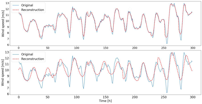Figure 3: Reconstructions of original signal. Top plot shows reconstruction with patch size 12 and close approximation of original signal. Only high-frequency fluctuations are not captured. Bottom plot shows low-frequency component reconstruction resulting from patch size 60.

3. RESULTS

Based on the trained dictionaries, we reconstructed the original data by running the dictionaries in inference mode (see Figure 1b). Each patch applied to the dictionary resulted in a sparse spiking activity (see [7] for details on leaky-integrate and fire neuron implemented in SAILnet). The reconstructed signal is the weighted sum of all dictionary elements with the weight being determined by the number of spikes per dictionary element. After the reconstruction, we performed unwhitening to transform the reconstruction to the mean and standard deviation of the original patch. For sake of demonstration we are showing two reconstructed signals in Figure 3 (sequence zoomed in to first 300 hours). For the dictionary trained with patch size 12 we can observe a fairly close reconstruction of the original signal, concluding that the dictionary learning algorithm is capable of capturing a diverse set of descriptive features from the applied training data. For the dictionary trained with patch size 60 we can observe that higher frequency components are not present in the reconstruction as the corresponding atoms adopted to lower frequency patterns.

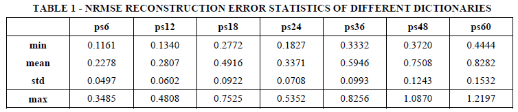
To evaluate the different dictionaries more quantitatively, and to better understand qualitative differences between the different dictionaries, we are comparing the respective reconstruction errors in Table 1. For this we randomly chose 1000 signals from the test set and calculated the normalized root mean square errors (NRMSE) for all dictionaries. As expected, shorter patch sizes maintaining higher frequency components allow for more accurate reconstructions of the original signals, while longer patch sizes exhibit higher reconstruction errors. Interestingly though, patch size is not directly linearly related to reconstruction accuracy. As can be observed, patch size of 18h does not provide improvement over patch size of 24h. For all measures it exhibits inferior reconstruction accuracies.

Figure 4: Coherence analysis of different dictionaries (performed with scipy.signal.coherence function and parameter nperseg=120; all other parameters used with their default values). Shorter patch sizes allow reconstructions maintaining coherence over a wider frequency spectrum, while longer patch sizes cut off higher frequencies more quickly. It can be observed that the filter behaviors of most dictionaries are tuned to specific wind cycles like 24h or 12h (see vertical lines indicating “wave length'”). All dictionaries have low coherence for rapid changes in wind speed (high frequencies).

We further investigated the filtering behavior of dictionaries by performing a coherence analysis between the original and the reconstructed signals. Coherence is a similarity measure of two signals as a function of their frequency components. Here, coherence expresses the similarity in the power spectrum between the original and the reconstructed signals. Coherence is bound in the interval [0, 1] from zero to full similarity. We selected 1000 random signals from the test set and performed the coherence analysis for all dictionaries. Coherence results for each dictionary are expressed as the respective average across all 1000 signals. Results of the coherence analysis can be seen in Figure 4. In a general sense, the shown coherence plot confirms two initial assumptions: first, different dictionaries lead to different reconstructions (with specific frequency components filtered out) and second, the transfer functions  are more complex than simple low or band pass filters. While detecting a clear drop in coherence past 0.2 cycles per hour, short patch sizes maintain some coherence with the original signal implying the theoretical possibility to reconstruct higher frequency behavior. This was already qualitatively observed in Figure 3. Longer patch sizes already lead to a clear and consistent drop in coherence past 0.1 cycles per hour. The second aspect, the transfer function of a dictionary, shows some multi-band pass behavior for most dictionaries. While patch size 6 still somewhat resembles a low pass filter, all other dictionaries more clearly exhibit selectivity to a set of frequency components. As indicated in the coherence plot, most notable frequencies captured are with wavelengths of 24h, 12h, 8h and 6h.

As our dictionaries were learned directly from data we verify if the coherence patterns are related to frequencies found in the actual data. In Figure 5 we demonstrate the Fast Fourier Transform (FFT) of a time series from the original dataset. It can be observed that the coherences from Figure 4 are closely related to the actual frequency components found in the data. This indicates the ability of dictionaries to be learned as filters tuned to the most prevalent frequencies within the data.

Figure 5: Fast Fourier Transform of a wind speed time series. Vertical lines indicate wavelengths. Peaks indicate strong daily and half-daily wind patterns.

4. DISCUSSION

In the introduction of this paper we have briefly discussed STL decomposition and its limited ability to detect more complex patterns. Decomposition has as its goal to extract deterministic patterns and separate random fluctuations from the data. However, for complex signals the remainder of the decomposition often represents a major part. DL allows to closely reconstructing complex signals with minimum error. This has two implications. First, by choice of the dictionary the reconstruction error (or remainder) can be lowered in magnitude in comparison to the overall signal amplitude. And second, reconstructing signals is a deterministic process based on linear combinations of known features. Utilizing multiple dictionaries with different filter characteristics (similar to ensemble learning methods) has the theoretical potential to further improve decomposition results. An application of ensemble methods to time series forecasting has recently been presented in [12].

Another potential application of decomposition through dictionaries is forecasting. Decomposition is often performed to simplify forecasting. DL offers the possibility to transform the challenge into forecasting a sparse signal representation. Rather than forecasting the actual signal, one could forecast the sparse spike patterns generated by the dictionaries. [13] described that through such a neocortical encoding of activity forecasting becomes linearly decodable. A problem as pointed out in [14] might arise from the sparse, seemingly random activity patterns of individual neurons. Known activity correlations between neurons over a relevant time span might alleviate this potential problem.

5. CONCLUSION

Despite decades of research, across various engineering and scientific disciplines, time series analysis often remains a daunting task. This can be reasoned about from various perspectives. For one, it is a question of separating real data from noise. Decomposition aims at separating composite time series into more easily analyzable components on the one side and noise on the other. However, it is rarely obvious to affirm that remainders of decompositions are purely noise and do not contain any more information that could aid in the overall analysis. Another perspective is that of representation. Depending on the domain one either decomposes or transforms in, i.e., the frequency domain to better analyze a signal. But every decomposition or transformation provides some insights while it obscures others. Ultimately it is a question of finding a good match between representation and application challenges. Here we have presented temporal DL as a method for creating different decompositions from time series signals. We have adopted an existing DL algorithm to learn temporal receptive fields. By training a variety of dictionaries with different TRF lengths, we have shown the ability for a given dictionary to learn specific patterns inherent in the data. The ability to directly learn features from data, contrary to using fixed mathematical kernel functions, provides the theoretical possibility to better separate noise from data. This hypothesis was supported by performing a coherence analysis between original signals and their dictionary dependent reconstructions. The coherence analysis has shown how shorter patch sizes maintain coherence over a wider frequency range while longer patch sizes function more selectively to a set of lower frequencies found in the data. This was shown exemplary on reconstructions with two different dictionaries. Relevant for future research, DL allows creating ensembles of deterministic and sparse representations of dense time series signals with, depending on the patch size, very low reconstruction errors. Such deterministic, sparse representations might open up new directions for analysis and processing of time series signals. We therefore stress the significance of this paper as contributing to new directions for methodological development in time series analysis.

6. REFERENCES

[1] Y. LeCun, Y. Bengio, and G. Hinton, “Deep learning,” Nature, vol. 521, no. 7553, p. 436, 2015.

[2] M. S. Lewicki and T. J. Sejnowski, “Learning Overcomplete Representations,” Neural Computation,   vol. 12, no. 2, pp. 337–365, 2000.

[4] J. Mairal, F. Bach, J. Ponce, and G. Sapiro, “Online Dictionary Learning for Sparse Coding,” in Proceedings of the 26th Annual International Conference on Machine Learning, ACM, 2009, pp. 689–         696.

[5] J. Fritz, S. Shamma, M. Elhilali, and D. Klein, “Rapid task-related plasticity of spectrotemporal receptive fields in primary auditory cortex,” Nature Neuroscience, vol. 6, no. 11, p. 1216, 2003.

[6] Q. Barthélemy, C. Gouy-Pailler, Y. Isaac, A. Souloumiac, A. Larue, and J. I. Mars, “Multivariate Temporal Dictionary Learning for EEG,” Journal of Neuroscience Methods, vol. 215, no. 1, pp. 19–28, 2013.

[7] J. Zylberberg, J. T. Murphy, and M. R. DeWeese, “A Sparse Coding Model with Synaptically Local Plasticity and Spiking Neurons Can Account for the Diverse Shapes of V1 Simple Cell Receptive Fields,” PLoS Computational Biology, vol. 7, no. 10, e1002250, 2011.

[8] S. Saha, S. Moorthi, X. Wu, J. Wang, S. Nadiga, P. Tripp, D. Behringer, Y.-T. Hou, H.-y. Chuang, M. Iredell, et al., “The NCEP Climate Forecast System Version 2,” Journal of Climate, vol. 27, no. 6, pp. 2185–2208, 2014.

[9] S. Dasgupta, F. Wörgötter, and P. Manoonpong, “Information Theoretic Self-organised Adaptation in Reservoirs for Temporal Memory Tasks,” in International Conference on Engineering Applications of  Neural Networks, Springer, 2012, pp. 31–40.

[10] N. A. Lesica and B. Grothe, “Efficient Temporal Processing of Naturalistic Sounds,” PloS One, vol. 3, no.2, e1655, 2008.

[11] K. Patil, D. Pressnitzer, S. Shamma, and M. Elhilali, “Music in Our Ears: The Biological Bases of Musical Timbre Perception,” PLoS Computational Biology, vol. 8, no. 11, e1002759, 2012.

[12] P. Laurinec, M. Lóderer, M. Lucká, and V. Rozinajová, “Density-based unsupervised ensemble learning methods for time series forecasting of aggregated or clustered electricity consumption,”  Journal of Intelligent Information Systems, pp. 1–21, 2019.

[14] A. Longtin, “Nonlinear Forecasting of Spike Trains from Sensory Neurons,” International Journal of Bifurcation and Chaos, vol. 3, no. 03, pp. 651–661, 1993.