<?xml version="1.0" encoding="ISO-8859-1"?><article xmlns:mml="http://www.w3.org/1998/Math/MathML" xmlns:xlink="http://www.w3.org/1999/xlink" xmlns:xsi="http://www.w3.org/2001/XMLSchema-instance">
<front>
<journal-meta>
<journal-id>2518-4431</journal-id>
<journal-title><![CDATA[Investigación & Desarrollo]]></journal-title>
<abbrev-journal-title><![CDATA[Inv. y Des.]]></abbrev-journal-title>
<issn>2518-4431</issn>
<publisher>
<publisher-name><![CDATA[UNIVERSIDAD PRIVADA BOLIVIANA]]></publisher-name>
</publisher>
</journal-meta>
<article-meta>
<article-id>S2518-44312017000200002</article-id>
<title-group>
<article-title xml:lang="en"><![CDATA[THE GROWTH OF WORLD TRADE: THE ROBUSTNESS OF THE EVIDENCE]]></article-title>
<article-title xml:lang="es"><![CDATA[EL CRECIMIENTO DEL COMERCIO MUNDIAL: LA SOLIDEZ DE LA EVIDENCIA]]></article-title>
</title-group>
<contrib-group>
<contrib contrib-type="author">
<name>
<surname><![CDATA[Montero Ledezma]]></surname>
<given-names><![CDATA[Paola L.]]></given-names>
</name>
<xref ref-type="aff" rid="A01"/>
</contrib>
</contrib-group>
<aff id="A01">
<institution><![CDATA[,Universidad Privada Boliviana Centro de Generación de Información y Estadística (CEGIE) ]]></institution>
<addr-line><![CDATA[ ]]></addr-line>
</aff>
<pub-date pub-type="pub">
<day>00</day>
<month>00</month>
<year>2017</year>
</pub-date>
<pub-date pub-type="epub">
<day>00</day>
<month>00</month>
<year>2017</year>
</pub-date>
<volume>2</volume>
<numero>17</numero>
<fpage>5</fpage>
<lpage>19</lpage>
<copyright-statement/>
<copyright-year/>
<self-uri xlink:href="http://www.scielo.org.bo/scielo.php?script=sci_arttext&amp;pid=S2518-44312017000200002&amp;lng=en&amp;nrm=iso"></self-uri><self-uri xlink:href="http://www.scielo.org.bo/scielo.php?script=sci_abstract&amp;pid=S2518-44312017000200002&amp;lng=en&amp;nrm=iso"></self-uri><self-uri xlink:href="http://www.scielo.org.bo/scielo.php?script=sci_pdf&amp;pid=S2518-44312017000200002&amp;lng=en&amp;nrm=iso"></self-uri><abstract abstract-type="short" xml:lang="en"><p><![CDATA[In this work we revisit the seminal paper “The growth of world trade: tariffs, transport costs, and income similarity” by S. Baier and J. Bergstrand published in the Journal of International Economics (2001). We develop a rigorous econometric analysis of the robustness of their results. While our findings support Baier and Bergstrand (2001)’s general conclusions, we provide refined evidence of the results. Under robust estimators, we show that the presence of outliers overestimated the effect of trade liberalization and underestimated the effect of income growth, as sources of world trade growth in the second half of the past century.]]></p></abstract>
<abstract abstract-type="short" xml:lang="es"><p><![CDATA[En este trabajo revisamos el influyente artículo “The growth of world trade: tariffs, transport costs, and income similarity” de S. Baier y J. Bergstrand publicado en el Journal of International Economics (2001). Desarrollamos un análisis econométrico riguroso de la solidez de sus resultados. Si bien nuestros hallazgos respaldan las conclusiones generales de Baier y Bergstrand de 2001, proporcionamos evidencia depurada de los resultados. Bajo estimadores robustos, mostramos que la presencia de valores atípicos sobreestimó el efecto de la liberalización del comercio y subestimó el efecto del crecimiento del ingreso como fuentes del crecimiento del comercio mundial en la segunda mitad del siglo pasado.]]></p></abstract>
<kwd-group>
<kwd lng="en"><![CDATA[Gravity Equation]]></kwd>
<kwd lng="en"><![CDATA[Robustness]]></kwd>
<kwd lng="en"><![CDATA[Outliers Detection]]></kwd>
<kwd lng="es"><![CDATA[Modelo de Gravedad]]></kwd>
<kwd lng="es"><![CDATA[Robustez]]></kwd>
<kwd lng="es"><![CDATA[Identificación de Valores Atípicos]]></kwd>
</kwd-group>
</article-meta>
</front><body><![CDATA[ <p align=left><font color="#800000" size="2" face="Verdana, Arial, Helvetica, sans-serif">http://dx.doi.org/10.23881/idupbo.017.2-1e</font></p>     <p align=right><font size="2" face="Verdana, Arial, Helvetica, sans-serif"><b>ART&Iacute;CULOS &ndash; ECONOMIA Y EMPRESA</b></font></p>     <p align=right>&nbsp;</p>     <p align=center><font size="4" face="Verdana, Arial, Helvetica, sans-serif"><b>THE GROWTH OF WORLD TRADE: THE ROBUSTNESS OF   THE EVIDENCE</b></font></p>     <p align=center><font size="2" face="Verdana, Arial, Helvetica, sans-serif"><b>&nbsp;</b></font><font size="2" face="Verdana, Arial, Helvetica, sans-serif"><b>&nbsp;</b></font></p>      <p align=center><font size="3" face="Verdana, Arial, Helvetica, sans-serif"><b>EL CRECIMIENTO DEL COMERCIO MUNDIAL: LA SOLIDEZ DE LA EVIDENCIA</b></font></p>     <p align=center>&nbsp;</p>     <p align=center><font size="2" face="Verdana, Arial, Helvetica, sans-serif"><b>&nbsp;</b></font></p>     <p align=center><font size="2" face="Verdana, Arial, Helvetica, sans-serif"><b>Paola L. Montero Ledezma&nbsp;</b></font></p>      <p align=center><font size="2" face="Verdana, Arial, Helvetica, sans-serif"><i>Centro de Generación de Información y Estadística </i>(CEGIE)</font></p>      ]]></body>
<body><![CDATA[<p align=center><font size="2" face="Verdana, Arial, Helvetica, sans-serif"><i>Universidad Privada Boliviana</i></font></p>      <p align=center><font size="2" face="Verdana, Arial, Helvetica, sans-serif"><a href="mailto:paolamontero@lp.upb.edu">paolamontero@lp.upb.edu</a></font></p>      <p align=center><font size="2" face="Verdana, Arial, Helvetica, sans-serif">(Recibido el 20 noviembre 2017, aceptado para publicación el 12 diciembre 2017)</font></p>     <p align=center>&nbsp;</p>     <p align=center>&nbsp;</p> <hr noshade>     <p align=justify><font size="2" face="Verdana, Arial, Helvetica, sans-serif"><b>ABSTRACT</b></font></p>      <p align="justify"><font size="2" face="Verdana, Arial, Helvetica, sans-serif">In this work we revisit the seminal paper “The growth of world trade: tariffs, transport costs, and income similarity” by S. Baier and J. Bergstrand published in the <i>Journal of International Economics </i>(2001). We develop a rigorous econometric analysis of the robustness of their results. While our findings support Baier and Bergstrand (2001)’s general conclusions, we provide refined evidence of the results. Under robust estimators, we show that the presence of outliers overestimated the effect of trade liberalization and underestimated the effect of income growth, as sources of world trade growth in the second half of the past century.</font></p>      <p align=justify><font size="2" face="Verdana, Arial, Helvetica, sans-serif"><b>Keywords:</b> Gravity Equation, Robustness, Outliers Detection.</font></p>  <hr noshade>     <p align=justify><font size="2" face="Verdana, Arial, Helvetica, sans-serif"><b>RESUMEN</b></font><font size="2" face="Verdana, Arial, Helvetica, sans-serif"><b>&nbsp;</b></font></p>     <p align="justify"><font size="2" face="Verdana, Arial, Helvetica, sans-serif">En este trabajo revisamos el influyente artículo “The growth of world trade: tariffs, transport costs, and income similarity” de S. Baier y J. Bergstrand publicado en el <i>Journal of International Economics</i> (2001). Desarrollamos un análisis econométrico riguroso de la solidez de sus resultados. Si bien nuestros hallazgos respaldan las conclusiones generales de Baier y Bergstrand de 2001, proporcionamos evidencia depurada de los resultados. Bajo estimadores robustos, mostramos que la presencia de valores atípicos sobreestimó el efecto de la liberalización del comercio y subestimó el efecto del crecimiento del ingreso como fuentes del crecimiento del comercio mundial en la segunda mitad del siglo pasado.</font></p>      ]]></body>
<body><![CDATA[<p align="justify"><font size="2" face="Verdana, Arial, Helvetica, sans-serif"><b>Palabras clave:</b> Modelo de Gravedad, Robustez, Identificación de Valores Atípicos.</font></p>  <hr noshade>     <p align="justify">&nbsp;</p>      <p align="justify">&nbsp;</p>      <p align="justify"><font size="3" face="Verdana, Arial, Helvetica, sans-serif"><b>1. INTRODUCTION </b></font></p>      <p align="justify"><font size="2" face="Verdana, Arial, Helvetica, sans-serif">“Why has world trade grown?” The question raised by the Nobel Prize Laureate Paul Krugman [2] has had different reactions over the years. The following stands are clearly identified. Journalists argue that world trade’s growth is a response to technological progress (transport costs reduction, economists support the idea of liberalization as the main drive, and [3] and [4] argue in favor of income convergence.</font></p>      <p align="justify"><font size="2" face="Verdana, Arial, Helvetica, sans-serif">Several papers have balanced the discussion in one way or another. Baier and Bergstrand [1] (henceforth BB (2001)), with over one thousand citations, bring an interesting econometric approach. The authors disentangle the relative effects of transport-cost reductions, tariff liberalization, and income convergence on the growth of world trade among several countries members of the Organization for Economic Cooperation and Development (OECD) between the late 1950s and the late 1980s. The main conclusion of their paper indicates ‘bilateral income growth explains about 67%, tariff-rate reductions about 25%, transport-cost declines about 8%, and income convergence represents virtually none of the average world trade growth.’ The importance of these findings in the trade literature leads us to deepen our understanding of this seminal paper.</font></p>      <p align="justify"><font size="2" face="Verdana, Arial, Helvetica, sans-serif">The aim of the present work is to revisit BB (2001)’s main results under the magnifier glass of several robustness tests. For this purpose, we describe a step-by-step methodology to test the robustness of cross-sectional data utilizing graphical detection of outliers as well as high breakdown point estimators. Under various methodologies we find that BB (2001)’s outcomes are sensitive to the presence of atypical points. More importantly, the share attributed to tariffs falls has been overestimated by seven percentage points and income growth has been underestimated by ten percentage points.</font></p>      <p align="justify"><font size="2" face="Verdana, Arial, Helvetica, sans-serif">Many have attempted to answer Krugman’s question. There is a vast literature on trade starting with [5] among others. For useful surveys see [6], [7], [8], [9]. Deepening on this literature, however, is beyond the scope of this paper. Therefore, we invite the curious reader to refer to the cited references if interested.</font></p>      <p align="justify"><font size="2" face="Verdana, Arial, Helvetica, sans-serif">From the empirical viewpoint, estimating a model by means of least-squares (LS) assumes certain behavior of observations in line with an econometric model. However, in a given sample not all observations are well behaved, there might be outliers: an observation which exists at an atypical distance from other observations in a random sample from a population. If the model does not consider these atypical observations, classical methods may yield biased coefficients and standard errors. The existence of outliers is a common problem in applied research, since their presence is not known beforehand.</font></p>      <p align="justify"><font size="2" face="Verdana, Arial, Helvetica, sans-serif">Outliers are classified into three categories: vertical outliers, good, and bad leverage points [10]. A vertical outlier is an observation whose dependent variable, <i>y</i>-dimension, is off the general trend of the rest of the data. A leverage point is an observation with an extreme value in the space of the explanatory variables, <i>x</i>-dimension. Leverage is a measure of how far an independent variable deviates from its mean. Leverage points are considered ‘good’ if they are located closely around the regression hyperplane, and ‘bad’ if they are outside of it. While bad leverage points have an important influence on the estimation of all coefficients, vertical outliers affect mostly the intercept of the regression. Moreover, they influence the slope of coefficients lightly. Finally, the effect of good leverage points is practically negligible on all coefficients [11].</font></p>      ]]></body>
<body><![CDATA[<p align="justify"><font size="2" face="Verdana, Arial, Helvetica, sans-serif">Applied researchers have warned us about the effects and implications of outliers in a sample. See an overview of the literature in [12]. Among those dedicated to study vertical outliers and bad leverage points are [13], [14], and [15] for theoretical insights as well as practical applications. Good leverage points have been largely ignored. However, [16] and [17] argue that good leverage points could yield underestimated standard errors and an overestimation of the <i>R</i>-squared. [18] addresses these problems by suggesting measures to ensure the robustness of the goodness-of-fit of a model.</font></p>      <p align="justify"><font size="2" face="Verdana, Arial, Helvetica, sans-serif">This paper is structured as follows. In section 2 we explain BB (2001)’s empirical model and provide a description of the data set used. In section 3 we discuss the detection of outliers and the different methodologies to solve this problem. The empirical results are presented in section 4, where we feature the analysis of the outliers identified by several methodologies. We also compare these results with the original regression. Section 5 concludes.</font></p>      <p align="justify">&nbsp;</p>      <p align="justify"><font size="3" face="Verdana, Arial, Helvetica, sans-serif"><b>2. BAIER AND BERGSTRAND (2001)</b></font></p>      <p align="justify"><font size="2" face="Verdana, Arial, Helvetica, sans-serif"><b>&nbsp;</b></font></p>      <p align="justify"><font size="2" face="Verdana, Arial, Helvetica, sans-serif">In this section we briefly review the most important features of the gravity equation, followed by BB (2001)’s econometric specification. After a description of the data, we reproduce BB (2001)’s outcomes.</font></p>      <p align="justify"><font size="2" face="Verdana, Arial, Helvetica, sans-serif">A standard framework to study the pattern of trade is the gravity model [19]. The idea is ‘to relate the value of bilateral flows to national income, population, distance, and contiguity’ (p. 8). The gravity equation is a log-linear cross-sectional specification that relates the nominal bilateral trade flow from exporter <i>i</i> to importer <i>j</i> in any year (<i>PX<sub>ij</sub></i>) to the exporting and importing countries’ nominal gross domestic products (<i>GDP<sub>i</sub></i> and <i>GDP<sub>j</sub></i>, respectively), distance between their economic center (<i>D<sub>ij</sub></i>) and a set of dummy variables intended to reflect the existence or not of preferential trading agreement (<i>PTA<sub>ij</sub></i>) or of a common frontier (<i>A<sub>ij</sub></i>). The basic gravity equation has the following econometric specification:<a href="#_ftn1" name="_ftnref1" title=""><sup><sup>[1]</sup></sup></a></font><font size="2" face="Verdana, Arial, Helvetica, sans-serif"><sup>&nbsp;</sup></font></p>      <p align=center><img src="/img/revistas/riyd/v2n17/a02_ecuacion_01.gif" width="771" height="46"></p>     <p align="justify"><font size="2" face="Verdana, Arial, Helvetica, sans-serif">where <i>e</i> is the natural logarithm base and <i>&#949;<sub>ij</sub></i> is a log-normally distributed error term.</font></p>      <p align="justify"><font size="2" face="Verdana, Arial, Helvetica, sans-serif">The empirical literature in international trade uses the typical gravity equation, whilst the novelty comes from the econometric specification as it is the case in BB (2001). In their econometric model they aim to evaluate the absolute and relative roles of real income growth, real income convergence, tariff reductions, and reductions in transportation costs, in explaining the growth of world trade between the late 1950s and the late 1980s.</font></p>      ]]></body>
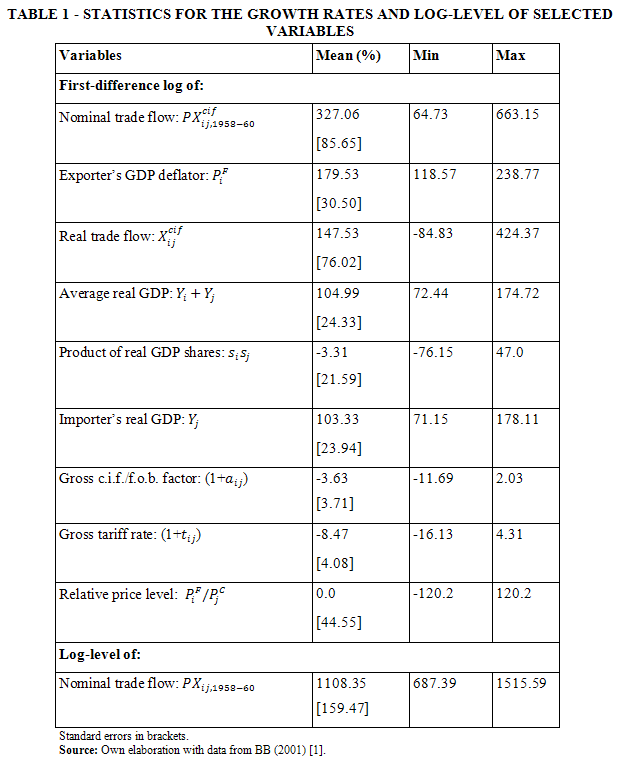
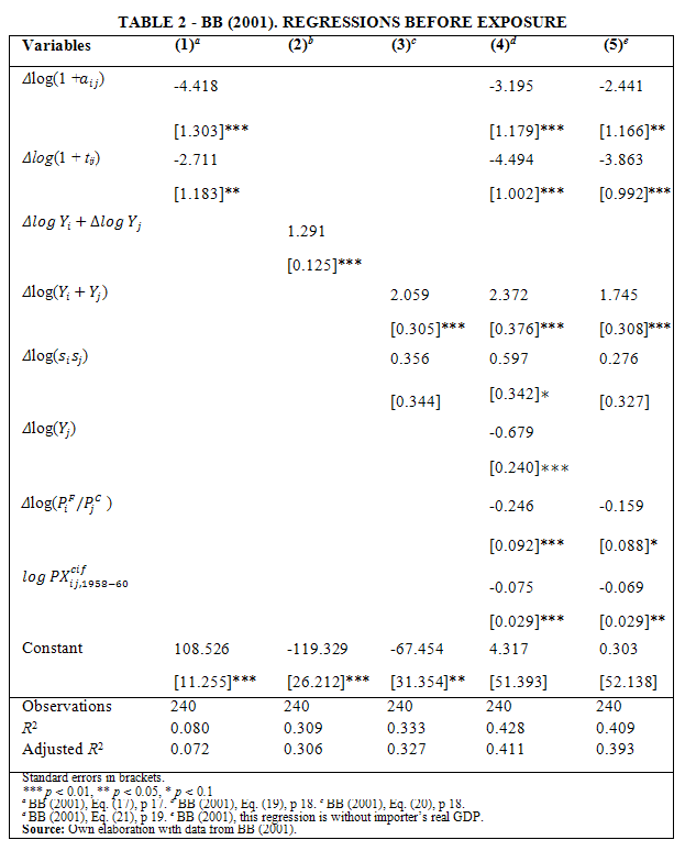
<body><![CDATA[<p align="justify"><font size="2" face="Verdana, Arial, Helvetica, sans-serif">The econometric model used in BB (2001) comes as a result of a general equilibrium model.<a href="#_ftn2" name="_ftnref2" title=""><sup><sup>[2]</sup></sup></a> It develops a gravity equation with the following specification:</font></p>     <p align="center"><img src="/img/revistas/riyd/v2n17/a02_ecuacion_02.gif" width="773" height="70"></p>     <p align=justify><font size="2" face="Verdana, Arial, Helvetica, sans-serif">Eq. (2) is a reproduction of BB (2001)’s Eq. (16), where variables are in a first-difference logarithmic form and nominal trade flows are deflated by a price index (<img src="/img/revistas/riyd/v2n17/a02_e004.gif" width=13 height=16 align="absmiddle">).<a href="#_ftn3" name="_ftnref3" title=""><sup><sup>[3]</sup></sup></a> On the purpose of studying growth, all variables are in real terms. The dependent variable, <img src="/img/revistas/riyd/v2n17/a02_e005.gif" width=23 height=20 align="absmiddle">, denotes the real trade flow (the nominal c.i.f. value of the trade flow divided by the exporter’s deflator). <img src="/img/revistas/riyd/v2n17/a02_e006.gif" width=8 height=12 align="absmiddle"><sub><i>i</i></sub> And <img src="/img/revistas/riyd/v2n17/a02_e006.gif" width=8 height=12 align="absmiddle"><sub><i>j</i></sub>, denote the real GDP of country<i> i </i>and<i> j </i>respectively; and <img src="/img/revistas/riyd/v2n17/a02_e008.gif" width=8 height=9 align="absmiddle">, <img src="/img/revistas/riyd/v2n17/a02_e009.gif" width=8 height=11 align="absbottom"> denote<i> i’s </i>and<i> j’s </i>share of the two countries real incomes.<a href="#_ftn4" name="_ftnref4" title=""><sup><sup>[4]</sup></sup></a> World income growth is captured in the constant. As explanatory variables one counts the effect of bilateral income growth, captured by variations in the term <img src="/img/revistas/riyd/v2n17/a02_e010.gif" width=34 height=14 align="absmiddle">. Since, <img src="/img/revistas/riyd/v2n17/a02_e011.gif" width=18 height=11 align="absmiddle"> is the product of real GDP shares, variation in <img src="/img/revistas/riyd/v2n17/a02_e011.gif" width=18 height=11 align="absmiddle"> represents the effect of income convergence. Therefore, the convergence of incomes of country pairs augments trade flow growth.<a href="#_ftn5" name="_ftnref5" title=""><sup><sup>[5]</sup></sup></a> Moreover, the effects of transport cost is captured by the gross c.i.f.-f.o.b. factor (1 + <img src="/img/revistas/riyd/v2n17/a02_e012.gif" width=14 height=11 align="absmiddle">), while the effect of tariff-rate changes is expressed by the gross tariff rate (1 + <img src="/img/revistas/riyd/v2n17/a02_e013.gif" width=12 height=13 align="absmiddle">). Linear constraints can be evaluated for coefficient estimates of <img src="/img/revistas/riyd/v2n17/a02_e014.gif" width=12 height=12 align="absmiddle"> and <img src="/img/revistas/riyd/v2n17/a02_e015.gif" width=12 height=12 align="absmiddle"> and nonlinear constraints for coefficient estimates of <img src="/img/revistas/riyd/v2n17/a02_e016.gif" width=12 height=12 align="absmiddle">, <img src="/img/revistas/riyd/v2n17/a02_e017.gif" width=12 height=12 align="absmiddle">, <img src="/img/revistas/riyd/v2n17/a02_e018.gif" width=12 height=12 align="absmiddle">, and <img src="/img/revistas/riyd/v2n17/a02_e019.gif" width=12 height=12 align="absmiddle">.</font></p>      <p align="justify"><font size="2" face="Verdana, Arial, Helvetica, sans-serif">BB (2001) assume that the elasticities of substitution in consumption (&#963;) and transformation of production (</font><font size="2">&gamma;</font><font size="2" face="Verdana, Arial, Helvetica, sans-serif">) are constant over the period of scrutiny. So, <img src="/img/revistas/riyd/v2n17/a02_e018.gif" width=12 height=12 align="absmiddle"> indicates whether or not the elasticity of transformation of output across markets is finite; if </font><font size="2">&gamma;</font><font size="2" face="Verdana, Arial, Helvetica, sans-serif"> = &#8734; as it is an standard assumption, <img src="/img/revistas/riyd/v2n17/a02_e020.gif" width=8 height=14 align="absmiddle">’s coefficient estimate will be 0. The variation in the countries’ relative price levels is denoted by <img src="/img/revistas/riyd/v2n17/a02_e021.gif" width=35 height=16 align="absmiddle">, where <img src="/img/revistas/riyd/v2n17/a02_e022.gif" width=13 height=16 align="absmiddle"> is the standard Dixit-Stiglitz price index of landed prices and <img src="/img/revistas/riyd/v2n17/a02_e023.gif" width=13 height=14 align="absmiddle"> is a CET index of the firms price. Provided that the initial trade period (1958 &#8722; 60) may have had some impact on the analysis, the full model to be estimated includes, in addition, the natural logarithm of the initial period’s trade flow level, log <img src="/img/revistas/riyd/v2n17/a02_e024.gif" width=64 height=20 align="absmiddle">. Last, <img src="/img/revistas/riyd/v2n17/a02_e025.gif" width=12 height=11 align="absmiddle"> is a normally distributed random error term. </font></p>      <p align="justify"><font size="2" face="Verdana, Arial, Helvetica, sans-serif">We use data from BB (2001), whose primarily source is the International Monetary Fund, International Financial Statistics 1995. The data set counts 240 observations and constitutes cross bilateral trade flows and economic characteristics among 16 countries belonging to the OECD. The countries are: Canada, United States, Japan, Belgium-Luxembourg, Denmark, France, Germany, Italy, Netherlands, United Kingdom, Austria, Norway, Sweden, Switzerland, Australia and Finland, here cited in decreasing order of c.i.f.-f.o.b. factors. Data is averaged over three years for the periods 1958 &#8722; 60 and 1986 &#8722; 88.</font></p>      <p align="justify"><font size="2" face="Verdana, Arial, Helvetica, sans-serif"><a href="#t1">Table 1</a> reports a summary of the mean, standard deviation, minimum and maximum values of the growth rate (i.e., logarithmic difference) of each of the variables and the log-level of the initial period’s trade flow. For instance, in 28 years the real trade flow has grown on average 148 percentage points.</font></p>      <p align="justify"><font size="2" face="Verdana, Arial, Helvetica, sans-serif">The results of different specifications of BB (2001)’s model are presented in <a href="#t2">Table 2</a>, in which the dependent variable is the real bilateral trade flows from 1958 &#8722; 60 to 1986 &#8722; 88, <img src="/img/revistas/riyd/v2n17/a02_e026.gif" width=31 height=20 align="absmiddle"> between the countries<i> i </i>and<i> j</i>. We use ordinary least squares (LS) for all the columns. Column (1) includes as explanatory variables changes in the gross c.i.f.-f.o.b. factors and gross tariff rates over the indicated period. As expected, reducing transportation costs and tariff rates increase the growth of world trade; although the regression goodness is only 7% (adjusted <i>R</i><sup>2</sup> = 0<i>.</i>07). Indeed, this regression lacks of bilateral income growth as an explanatory variable.</font></p>      <p align="justify"><font size="2" face="Verdana, Arial, Helvetica, sans-serif">One can begin to understand how much each variable explains of the real bilateral trade flows. For instance, multiplying the mean of the first-difference log of the gross tariff rate (-8.47) times its coefficient (-2.711) yields 23 percentage points. That means, it explains 16% of the real bilateral trade flows growth.<a href="#_ftn6" name="_ftnref6" title=""><sup><sup>[6]</sup></sup></a> Through similar computations, the mean of the first-difference log of the gross c.i.f.-f.o.b. factors explains 11% of the bilateral trade flow growth.</font><font size="2" face="Verdana, Arial, Helvetica, sans-serif"><b>&nbsp;</b></font></p>      <p align="justify"><font size="2" face="Verdana, Arial, Helvetica, sans-serif">Column (2) presents the estimation of a ‘frictionless’ model, which is without tariffs, transportation costs, and distribution costs [20]. This model assumes complete specialization of each country in the production of one good, whose prices are normalized to unity. The gravity equation is the result of an expenditure system combined with identical homothetic preferences, and the specialization of each country in one good. Despite of improvements to the Anderson’s model to overcome the limited number of countries [21, 22, 27], other limitations persist, i.e., geographical considerations, transportation costs, tariff barriers. The simplicity of this model does not prevent it from reaching a higher goodness-of-fit than the previous model, with 31% of goodness (adjusted <i>R</i><sup>2</sup> = 0<i>.</i>31). The world output growth is 119%, and the coefficient estimate of both countries income growth is close to unity. Column (3) is also a ‘frictionless’ model but decomposing the income growth (&#916;log(<i>Y<sub>i</sub></i> + <i>Y<sub>j</sub></i>)) and the income convergence effects (&#916;log(<i>s<sub>i</sub>s<sub>j</sub></i>)). The regression goodness is slightly higher compared to the model in Column (2) (adjusted <i>R</i><sup>2</sup> = 0<i>.</i>33).</font><font size="2" face="Verdana, Arial, Helvetica, sans-serif"><b>&nbsp;</b></font></p>      <p align="justify"><font size="2" face="Verdana, Arial, Helvetica, sans-serif">The unrestricted model is presented in Column (4), which in addition to the variables in Column (3) includes transport costs, tariffs, average real GDP, income convergence, importers’ GDP, relative price level, and the natural logarithm of the initial period’s trade flow level. This regression has a greater explanatory power (adjusted <i>R</i><sup>2</sup> = 0<i>.</i>41) than Columns (1), (2), and (3). All coefficient estimates are statistically significant and identical to those presented in BB (2001, p 19), except for the constant. The signs of the coefficients are the expected and therefore consistent with the theoretical model. Studying these coefficients one can conclude that three factors contribute to explaining the 148 percentage points mean growth of trade; they are: bilateral income growth, tariff rate reductions, and falls in transport-cost.</font></p>      ]]></body>

<body><![CDATA[<p align="center"><font size="2" face="Verdana, Arial, Helvetica, sans-serif"><b>&nbsp;</b></font><a name="t1"></a><img src="/img/revistas/riyd/v2n17/a02_tabla_01.gif" width="621" height="766"></p>      <p align="justify"><font size="2" face="Verdana, Arial, Helvetica, sans-serif">We confirm BB (2001)’s outcomes regarding tariff-rate reductions which indeed explain 38 percentage points (or roughly 26%) of the trade’s growth.<a href="#_ftn7" name="_ftnref7" title=""><sup><sup>[7]</sup></sup></a> Similarly, transport-costs falls explain 12 percentage points (or roughly 8%) of the growth of trade.<a href="#_ftn8" name="_ftnref8" title=""><sup><sup>[8]</sup></sup></a></font><font size="2" face="Verdana, Arial, Helvetica, sans-serif"><sup>&nbsp;</sup></font></p>      <p align="justify"><font size="2" face="Verdana, Arial, Helvetica, sans-serif">Bilateral income growth, which is calculated by adding the remaining explanatory variables, justify about 94 percentage points<a href="#_ftn9" name="_ftnref9" title=""><sup><sup>[9]</sup></sup></a> (or 64% of the total) of the trade’s growth. This result differs from the one in BB (2001) by three percentage points due to the constant coefficient, which we do not included due to its lack of statistical significance. Income convergence, although significant, has indeed a negligible contribution to explaining the mean growth of trade in this sample.</font></p>      <p align="justify"><font size="2" face="Verdana, Arial, Helvetica, sans-serif">Finally, Column (5) takes into account theoretical considerations regarding elasticities of substitution in consumption and transformation of production, presented above. We regress all the variables of Column (4), except for the importer’s real GDP. Clearly, this regression is less suitable than the one in Column (4), with goodness-of-fit of only 39% (adjusted <i>R</i><sup>2</sup> = 0<i>.</i>39). Consequently, the model that better fits the data and the one that we will further study is represented in Column (4).</font></p>      <p align="center"><a name="t2"></a><img src="/img/revistas/riyd/v2n17/a02_tabla_02.gif" width="623" height="774"></p>      <p align="justify">&nbsp;</p>     <p align="justify"><font size="3" face="Verdana, Arial, Helvetica, sans-serif"><b>3. METHODOLOGY AND THEORETICAL BACKGROUND</b></font><font size="2" face="Verdana, Arial, Helvetica, sans-serif"><b>&nbsp;</b></font></p>     <p align="justify"><font size="2" face="Verdana, Arial, Helvetica, sans-serif">In this section we use different methodologies suggested in the statistical and econometric literature to identify outliers and deal with them. Analyzing cross-sectional data, as stated in the Introduction, one can encounter three types of outlying observations. [10] calls them vertical outliers, good leverage points, and bad leverage points.</font></p>      <p align="justify"><font size="2" face="Verdana, Arial, Helvetica, sans-serif">In this paper, <i>vertical outliers</i> indicate those country-pairs with atypical bilateral real trade flows which are not atypical in the space of explanatory variables. Such observations might affect the coefficient of interest as well as the intercept. <i>Good leverage points</i> are atypical observations in the space of explanatory variables, but located close to the regression line. For instance, country-pairs with high trade flows and also highly integrated. Those observations raise the estimated standard errors and, thus, affect the statistical inference. Finally, <i>bad leverage points</i> are abnormal country-pairs in the space of explanatory variables and located far away from the true regression line. For example, country-pairs with low tariff rates and low bilateral trade flows. These points would affect coefficients and the intercept.</font></p>      <p align="justify"><font size="2" face="Verdana, Arial, Helvetica, sans-serif">A methodology to treat influential data consists on deleting the abnormal points one at a time, followed by the regression model using the <i>n</i> &#8722; 1 observations. Next, a comparison can be performed between the model with the total number of observations and the model with deleted observations. That difference provides a good idea of the influence of each atypical point deleted. To achieve this process, we must first identify the abnormal points. Here, we describe the different methodologies utilized. The classical tools are: the hat matrix, the externally and internally studentized residuals, difference in fits, difference in betas, Cook’s distance, Mahalanobis distance. Furthermore, the robust estimators are: S-estimators, MCD, Hadi, L-estimator, and MM-estimator. Let us define the model of interest as:</font></p>     ]]></body>
<body><![CDATA[<p align="center"><img src="/img/revistas/riyd/v2n17/a02_ecuacion_03.gif" width="773" height="46"></p>     <p align=justify><font size="2" face="Verdana, Arial, Helvetica, sans-serif">where <i>y</i> is the dependent variable, <i>X</i> is the vector of the explanatory variables, <i>&#946;</i> is the vector of regression parameters, <i>&#949;</i> is the error term, and <i>n</i> is the number of observations. As standard, errors are assumed to be independent of the explanatory variables and i.i.d., following a normal distribution <i>N</i>(0<i>, &#963;</i><sup>2</sup>). The coefficients are generally estimated by ordinary least square (LS):</font></p>      <p align="center"><img src="/img/revistas/riyd/v2n17/a02_ecuacion_04.gif" width="773" height="39"></p>      <p align=justify><font size="2" face="Verdana, Arial, Helvetica, sans-serif">or in matrix notation:</font></p>     <p align=center><img src="/img/revistas/riyd/v2n17/a02_e036.gif" width="110" height="15"></p>     <p align="justify"><font size="2" face="Verdana, Arial, Helvetica, sans-serif">At this point, we introduce the first method for outlier detection. The projection matrix, also known as the <i>hat matrix</i>,<a href="#_ftn10" name="_ftnref10" title=""><sup><sup>[10]</sup></sup></a> or the influence matrix [29] contains information about the influence of a data <i>y</i> value might have on each fitted <i>y</i> value (&#375;) [28, 30, 31]. By multiplying each side of Eq. (3) by <i>X</i>, we obtain the hat matrix, denoted <i>H</i>.</font></p>      <p align="center"><img src="/img/revistas/riyd/v2n17/a02_ecuacion_05.gif" width="769" height="49"></p>      <p align="justify"><font size="2" face="Verdana, Arial, Helvetica, sans-serif">where each fitted value is a (linear) combination of all the observed <i>y</i> values. That is:</font></p>      <p align=center><font size="2" face="Verdana, Arial, Helvetica, sans-serif">.</font><img src="/img/revistas/riyd/v2n17/a02_ecuacion_05_1.gif" width="209" height="24"></p>      <p align="justify"><font size="2" face="Verdana, Arial, Helvetica, sans-serif">Therefore, the larger the <img src="/img/revistas/riyd/v2n17/a02_e041.gif" width=14 height=14 align="absmiddle"> value, the more influence <img src="/img/revistas/riyd/v2n17/a02_e042.gif" width=10 height=9 align="absmiddle"> has on the fitted value [32]. The values <img src="/img/revistas/riyd/v2n17/a02_e043.gif" width=13 height=12 align="absmiddle"> form the hat matrix diagonal, which in case of being large it means that the <i>i<sup>th</sup></i> observation is influential. Let denote the sum of the diagonal values of the hat matrix as:</font></p>      ]]></body>
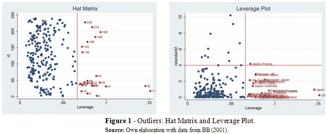
<body><![CDATA[<p align=center><img src="/img/revistas/riyd/v2n17/a02_ecuacion_05_2.gif" width="76" height="55"></p>      <p align="justify"><font size="2" face="Verdana, Arial, Helvetica, sans-serif">then, two rules of thumbs can be listed:</font></p>      <blockquote>       <p align="justify"><font size="2" face="Verdana, Arial, Helvetica, sans-serif">&#9679;&nbsp; If <img src="/img/revistas/riyd/v2n17/a02_e043.gif" width=13 height=12 align="absmiddle"> <i>&gt;</i> 2<i>p/n</i>, an observation might     be worth investigating [33].</font></p>       <p align="justify"><font size="2" face="Verdana, Arial, Helvetica, sans-serif">&#9679;&nbsp; If <img src="/img/revistas/riyd/v2n17/a02_e043.gif" width=13 height=12 align="absmiddle"> <i>&gt; </i>3<i>p/n</i>, the leverage is large [34].</font></p> </blockquote>     <p align="justify"><font size="2" face="Verdana, Arial, Helvetica, sans-serif">The best way to use the hat matrix diagonals is in a <i>leverage plot</i>. This plot puts the hat matrix diagonals on <i>x</i>-axis and the squared in standardized residuals on the <i>y</i>-axis (see <a href="#f1">Figure 1</a> for an application).</font></p>      <p align="justify"><font size="2" face="Verdana, Arial, Helvetica, sans-serif">[35] argue that having residuals with more than three or four standard deviations away from zero are potentially outliers. For this reason, a next step is to analyze standardized residuals (<img src="/img/revistas/riyd/v2n17/a02_e045.gif" width=25 height=12 align="absmiddle">) rather than raw residuals (<img src="/img/revistas/riyd/v2n17/a02_e046.gif" width=8 height=9 align="absmiddle">) [36]. For instance, an <i>internally studentized</i> <i>residual </i>is simple a standardized residual that writes:</font></p>      <p align=center><font size="2" face="Verdana, Arial, Helvetica, sans-serif"><img src="/img/revistas/riyd/v2n17/a02_e047.gif" width=69 height=23 align="absmiddle">          where      <img src="/img/revistas/riyd/v2n17/a02_e048.gif" width=69 height=13 align="absmiddle">         and        <img src="/img/revistas/riyd/v2n17/a02_e049.gif" width=124 height=14 align="absmiddle"></font></p>      <p align=justify><font size="2" face="Verdana, Arial, Helvetica, sans-serif">while <i>externally studentized residual</i> writes:</font></p>      <p align=center><font size="2" face="Verdana, Arial, Helvetica, sans-serif"><img width=82 height=24 src="/img/revistas/riyd/v2n17/a02_e050.gif">,</font></p>      ]]></body>
<body><![CDATA[<p align="justify"><font size="2" face="Verdana, Arial, Helvetica, sans-serif">where <img src="/img/revistas/riyd/v2n17/a02_e051.gif" width=17 height=15 align="absmiddle"> is an estimate of &sigma; when observation <i>i</i> is deleted. Both, internally and externally studentized residuals follow a <i>t</i>-distribution with <i>n</i> &#8722; <i>p</i> degrees of freedom [36].</font></p>      <p align="justify"><font size="2" face="Verdana, Arial, Helvetica, sans-serif">Note that <img src="/img/revistas/riyd/v2n17/a02_e042.gif" width=10 height=9 align="absmiddle"> is the observed response for the <i>i<sup>th</sup></i> observation. While <img src="/img/revistas/riyd/v2n17/a02_e053.gif" width=18 height=15 align="absmiddle"> is the predicted response for <i>i<sup>th</sup></i> observation based on the estimated model with the <i>i<sup>th</sup></i> observation deleted. Thus, the deleted residuals are <img src="/img/revistas/riyd/v2n17/a02_e054.gif" width=76 height=15 align="absmiddle">.</font></p>      <p align="justify"><font size="2" face="Verdana, Arial, Helvetica, sans-serif">The <i>difference in fits</i> is the number of standard deviations that the fitted value changes when the <i>i<sup>th</sup></i> case is omitted. It is defined as:</font></p>      <p align=center><font size="2" face="Verdana, Arial, Helvetica, sans-serif"><img width=89 height=28 src="/img/revistas/riyd/v2n17/a02_e055.gif">.</font></p>      <p align="justify"><font size="2" face="Verdana, Arial, Helvetica, sans-serif">An observation is regarded as influential if the absolute value of its <img src="/img/revistas/riyd/v2n17/a02_e056.gif" width=32 height=12 align="absmiddle"> value is greater than  <img src="/img/revistas/riyd/v2n17/a02_e057.gif" width=37 height=17 align="absmiddle"><i> </i>[32].</font></p>      <p align="justify"><font size="2" face="Verdana, Arial, Helvetica, sans-serif">The <i>difference in betas</i> indicates by how much an estimated parameter changes when one single observation is deleted. An observation is influential if the absolute value of its <img src="/img/revistas/riyd/v2n17/a02_e058.gif" width=66 height=16 align="absmiddle"> is greater than <img src="/img/revistas/riyd/v2n17/a02_e059.gif" width=29 height=15 align="absmiddle"> [32]. This indicator writes:</font></p>      <p align=center><font size="2" face="Verdana, Arial, Helvetica, sans-serif"><img src="/img/revistas/riyd/v2n17/a02_e060.gif" width=143 height=18 align="absmiddle">.</font></p>      <p align="justify"><font size="2" face="Verdana, Arial, Helvetica, sans-serif"><i>Cook’s Distance</i><a href="#_ftn11" name="_ftnref11" title=""><sup><sup>[11]</sup></sup></a> is used for measuring the influence of a data point when performing a LS regression analysis. It helps identify data points that require a checking for validity, or to spot the regions where more data points are needed. </font></p>      <p align=center><font size="2" face="Verdana, Arial, Helvetica, sans-serif"><img width=89 height=24 src="/img/revistas/riyd/v2n17/a02_e061.gif">.</font></p>      <p align="justify"><font size="2" face="Verdana, Arial, Helvetica, sans-serif"><i>D<sub>i</sub> </i>can be interpreted as “the scaled Euclidean distance between the two vectors of fitted values when the fitting is done by including or excluding the <i>i<sup>th</sup></i> observation.” [33, p 383]. The cut-off values for identifying influential points are widely discussed. [39] suggest <i>D<sub>i</sub></i> <i>&gt;</i> 1 as a cut-off point, while other authors indicated <i>D<sub>i</sub></i> <i>&gt;</i> 4<i>/n</i>, where <i>n</i> is the number of observations [40, 34].</font></p>      ]]></body>
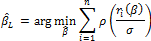
<body><![CDATA[<p align="justify"><font size="2" face="Verdana, Arial, Helvetica, sans-serif"><i>Mahalanobis distances</i>, first introduced in [41], are used to identify leverage in higher dimensions. The Mahalanobis distance of an observation  <img src="/img/revistas/riyd/v2n17/a02_e062.gif" width=130 height=16 align="absmiddle"> from a set of observations with mean <img src="/img/revistas/riyd/v2n17/a02_e063.gif" width=132 height=16 align="absmiddle"> and covariance matrix <img src="/img/revistas/riyd/v2n17/a02_e064.gif" width=6 height=9 align="bottom"> is defined as:</font></p>      <p align=center><font size="2" face="Verdana, Arial, Helvetica, sans-serif"><img width=173 height=17 src="/img/revistas/riyd/v2n17/a02_e065.gif">.</font></p>      <p align="justify"><font size="2" face="Verdana, Arial, Helvetica, sans-serif">However, <img src="/img/revistas/riyd/v2n17/a02_e066.gif" width=22 height=12 align="absmiddle"> are not robust since they are based on classical estimations, i.e., the mean <img src="/img/revistas/riyd/v2n17/a02_e067.gif" width=7 height=9 align="absmiddle"> and standard deviation <img src="/img/revistas/riyd/v2n17/a02_e064.gif" width=6 height=9 align="bottom">. Therefore, after some computations one can rewrite the Mahalanobis distance as:<a href="#_ftn12" name="_ftnref12" title=""><sup><sup>[12]</sup></sup></a></font></p>      <p align="center"><font size="2" face="Verdana, Arial, Helvetica, sans-serif"><img width=151 height=29 src="/img/revistas/riyd/v2n17/a02_e068.gif">.</font></p>      <p align="justify"><font size="2" face="Verdana, Arial, Helvetica, sans-serif">[42] suggests several critical values to identify atypical points. Here, we follow [32] and use <img src="/img/revistas/riyd/v2n17/a02_e069.gif" width=42 height=29 align="absmiddle">.</font></p>      <p align="justify"><font size="2" face="Verdana, Arial, Helvetica, sans-serif">Since, classical tools for outlier identification do not guarantee an appropriate recognition and resistance to all types of outliers, high breakdown point estimators are needed. Among the robust estimators we center on the S-estimators, Minimum Covariance Determinant, Hadi method.</font></p>      <p align="justify">&nbsp;</p>      <p align="justify"><font size="2" face="Verdana, Arial, Helvetica, sans-serif">The <i>S-estimator</i> stands out due to its strong robustness and asymptotic properties. The S-estimator’s objective is to minimize the sum of a function of the deviations [43]. In a nutshell, the S-estimator aims to minimize another measure of the dispersion of the residuals as a robust alternative to LS, that is:</font></p>      <p align=center><font size="2" face="Verdana, Arial, Helvetica, sans-serif"><img width=192 height=21 src="/img/revistas/riyd/v2n17/a02_e070.gif">.</font></p>      <p align="justify"><font size="2" face="Verdana, Arial, Helvetica, sans-serif">This estimator finds a regression line that minimizes a robust estimate of the scale of the residuals. It is highly resistant to leverage points, and it is robust to vertical outliers. However,  the S-estimators is known to be inefficient.</font></p>      ]]></body>
<body><![CDATA[<p align="justify"><font size="2" face="Verdana, Arial, Helvetica, sans-serif">[44] propose the <i>Minimum Covariance Determinant</i> estimator (henceforth, MCD). Based on [45]’s generalized variance. By seeking for the 50% subsample with the smallest generalized variance, and assuming that the subsample is outliers-free, the MCD estimator can hence be used to compute robust estimates.</font></p>      <p align="justify"><font size="2" face="Verdana, Arial, Helvetica, sans-serif">[46] proposes a novel detection procedure in presence of outliers. It consists on calculating the Mahalanobis distance, but using a vector of variable medians instead of a vector of means:</font></p>      <p align=center><font size="2" face="Verdana, Arial, Helvetica, sans-serif"><img width=220 height=17 src="/img/revistas/riyd/v2n17/a02_e071.gif">.</font></p>      <p align="justify"><font size="2" face="Verdana, Arial, Helvetica, sans-serif">The idea is to sort individuals by <img src="/img/revistas/riyd/v2n17/a02_e072.gif" width=27 height=14 align="absmiddle">, use the subsample with the first <i>p</i> + 1 points in order to re-estimate <i>µ</i> and &#931;. Next, one must recalculate <img src="/img/revistas/riyd/v2n17/a02_e072.gif" width=27 height=14 align="absmiddle"> and sort the data again. If the first point is an outlier one must repeat the process until the first point is no longer an outlier.</font></p>      <p align="justify"><font size="2" face="Verdana, Arial, Helvetica, sans-serif">Heretofore, we have described outlier detection methods whose limitation is to simply identify atypical points for their elimination. Next, we introduce methodologies which deal with outliers during the process of fitting the data to the model. Among this we explain the L-estimator, the M-estimator, and the MM-estimator.</font></p>      <p align="justify"><font size="2" face="Verdana, Arial, Helvetica, sans-serif">A problem with Eq.(4) consist on the excessive weight given to large residuals. LS is therefore sensitive to outliers. Several alternatives have been proposed. Let us begin with the <i>L-estimator</i> in which the squared function of residuals is replaced by its absolute value. That is:</font></p>      <p align=center><font size="2" face="Verdana, Arial, Helvetica, sans-serif"><img width=116 height=41 src="/img/revistas/riyd/v2n17/a02_e073.gif"></font></p>      <p align="justify"><font size="2" face="Verdana, Arial, Helvetica, sans-serif">The <i>M-estimator</i> introduced by [47], first awards a weight zero to individuals with Cook distances larger than 1.</font></p>      <p align=center><font size="2" face="Verdana, Arial, Helvetica, sans-serif"><img width=151 height=41 src="/img/revistas/riyd/v2n17/a02_e074.gif"></font></p>      <p align="justify"><font size="2" face="Verdana, Arial, Helvetica, sans-serif">Next, a “re-descending” M-estimator is computed using the iterative algorithm starting from a monotonic M-solution. Finally, <i>&#963;</i> is re-estimated at each iteration using the median residual of the previous iteration. This estimator’s procedure is based on iteratively reweighted least squares which work by assigning a weight to each observation and giving higher weight to better behaved observations<a href="#_ftn13" name="_ftnref13" title=""><sup><sup>[13]</sup></sup></a> [32]. This methodology, however, uses an initial estimate as initial point to compute the weights followed by iterations to re-weight the least squares algorithm. Consequently, full robustness analysis requires high breakdown point estimators such as MM-estimators.</font></p>      ]]></body>
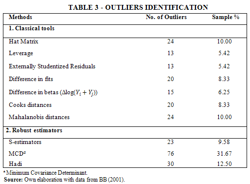
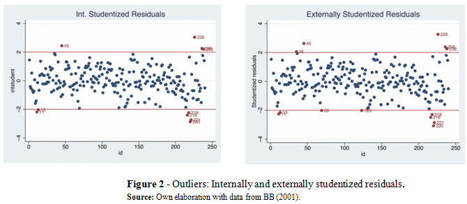
<body><![CDATA[<p align="justify"><font size="2" face="Verdana, Arial, Helvetica, sans-serif"><i>MM-estimators </i>attempt to retain both the robustness and resistance of S-estimation, and at the same time gain in effciency (as with the M-estimation). The procedure is the following: (i) it finds a highly robust and resistant S-estimate that minimizes the residuals; and (ii) it holds constant the estimated scale while a M-estimate is estimated.</font></p>     <p align="justify">&nbsp;</p>     <p align="justify"><font size="3" face="Verdana, Arial, Helvetica, sans-serif"><b>4. ANALYSIS</b></font></p>      <p align="justify"><font size="2" face="Verdana, Arial, Helvetica, sans-serif">We target the regression of <a href="#t2">Table 2</a>, Column (4), to check for the existence of outliers. We compare the results from the methodologies described in Section 3 to evaluate the robustness of these results. Following the same structure as in section 3, first, we go through classical tools for outliers’ identification. In this case, the percentage of outliers is between 5% and 10%. However, since these tools do not guarantee an appropriate identification and resistance to all types of outliers we move to robust estimators. Using high-break point estimators the sample presents between 10% and 32% of outliers depending on the method.</font></p>      <p align="justify"><font size="2" face="Verdana, Arial, Helvetica, sans-serif"><a href="#t3">Table 3</a> below summarizes these outcomes. Among the classical tools to identify abnormal points, leverage and externally studentized residuals hold the lowest number of outliers as a percentage of the sample. This is because in the leverage plot large outliers might mask smaller ones. For the case of difference in betas, we pick the coefficient of the income growth, only to find 6% of outliers. We reach the same results, 10% of outliers, with the hat matrix and Mahalanobis distances. Nevertheless, none of the classical tools succeed at detecting more than 24 outliers.</font></p>      <p align="justify"><font size="2" face="Verdana, Arial, Helvetica, sans-serif">There are more interesting results when we look at robust estimators. Among them, the MCD’s outcome calls for further scrutiny.</font></p>      <p align="justify"><font size="2" face="Verdana, Arial, Helvetica, sans-serif">&#9679;&nbsp; <b>Graphical detection of outliers</b></font></p>      <p align="justify"><font size="2" face="Verdana, Arial, Helvetica, sans-serif">Among the classical tools used for the identification of outliers, we begin with the hat matrix and the leverage plot, see <a href="#f1">Figure 1</a>. The observations plotted in red are leverage points; this is valid for all the following figures. The observations plotted in red are abnormal points. In both graphs, we identify the country-pairs of US-Japan (17) and Japan-US (32) as the points located furthest away from the rest of the sample.</font><font size="2" face="Verdana, Arial, Helvetica, sans-serif"><b>&nbsp;</b></font></p>      <p align="justify"><font size="2" face="Verdana, Arial, Helvetica, sans-serif">The internally and externally studentized residuals, presented in <a href="#f2">Figure 2</a> establish that the atypical country-pairs Japan-France (35), Japan-Finland (45), Finland-Canada (226), Finland-Austria (236), Finland-Sweden (238). Note that not all the country-pair outliers overlap.             </font></p>      <p align=center><a name="t3"></a><img src="/img/revistas/riyd/v2n17/a02_tabla_03.gif" width="514" height="377"></p>     ]]></body>
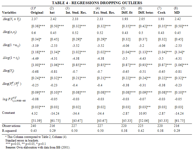
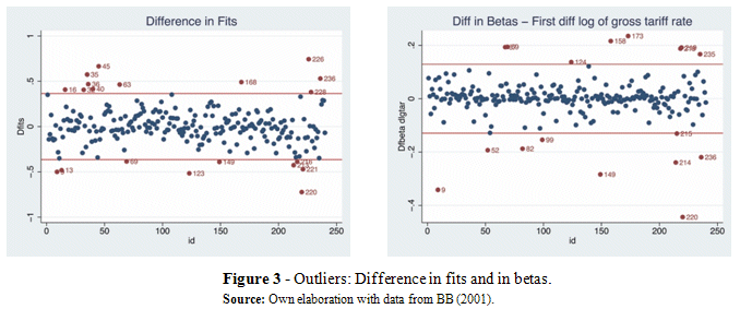
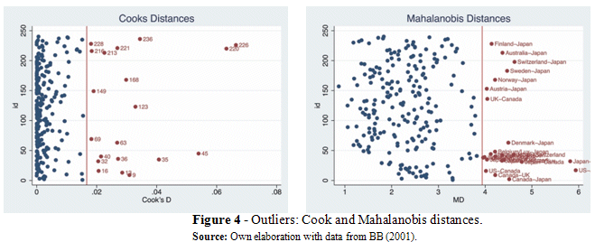
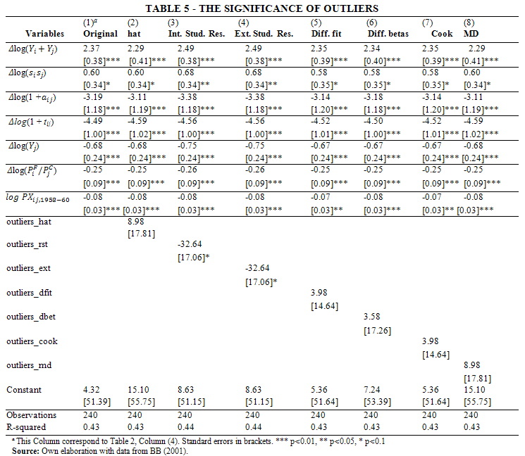
<body><![CDATA[<p align=center>&nbsp;</p>     <p align=center><a name="f1"></a><img src="/img/revistas/riyd/v2n17/a02_figure_01.gif" width="660" height="271"></p>     <p align=center>&nbsp;</p>     <p align=center><a name="f2"></a><img src="/img/revistas/riyd/v2n17/a02_figure_02.gif" width="670" height="293"></p>     <p align="justify"><font size="2" face="Verdana, Arial, Helvetica, sans-serif">The difference in fits reveals the country-pairs of Japan-Finland (45), Finland-Canada (226), Australia-UK (220) as outliers. We study the difference in betas applied to coefficient of income growth variable, log(<i>Y<sub>i</sub></i> + <i>Y<sub>j</sub></i>). The country-pairs that stick out are Australia-UK (220), Norway-Italy (173), among others (see <a href="#f3">Figure 3</a>).</font></p>     <p align="center"><a name="f3"></a><img src="/img/revistas/riyd/v2n17/a02_figure_03.gif" width="678" height="283"></p>     <p align="justify"><font size="2" face="Verdana, Arial, Helvetica, sans-serif">In <a href="#f4">Figure 4</a> we observe that according to the Cook’s distance, Australia-UK (220) and Finland-Canada (226) are the country-pairs with the highest distance from the rest of the sample. While Mahalanobis distance reveals even a higher number of outliers.</font></p>      <p align="center"><a name="f4"></a><img src="/img/revistas/riyd/v2n17/a02_figure_04.gif" width="659" height="268"></p>      <p align="justify"><font size="2" face="Verdana, Arial, Helvetica, sans-serif">Once outliers have been spotted, according to the criteria explained above, we regress the model of interest without those outliers and compare them. <a href="#t4">Table 4</a> provides a complete comparison of all the regressions. Column (1) reproduces Column (4) of <a href="#t2">Table 2</a>. Column (2) presents a regression without the outliers found with the hat matrix method. We observe that the <i>R</i><sup>2</sup> is much lower, with a value of 0.29. However, income convergence and the initial trade flow level are no longer significant. Similar results are given for Column (8), in which outliers have been pinpointed through Mahalanobis distance. The internally and externally studentized residuals yield more encouraging results, with an <i>R</i><sup>2</sup> = 0<i>.</i>50. However, the initial trade flow level lacks of significance. Dropping those outliers identified through difference in fits, difference in betas, and the Cook’s distance do not provide better goodness-of-fit (0<i>.</i>38 <i>&lt; R</i><sup>2</sup> <i>&lt;</i> 0<i>.</i>42). Moreover, income convergence and the initial trade flow level are not significant.</font></p>      <p align="justify"><font size="2" face="Verdana, Arial, Helvetica, sans-serif">The outcome of <a href="#t4">Table 4</a> is still unclear. Dropping a few outliers seems to deliver a higher goodness-of-fit, in some cases, but at a cost of losing significance in some explanatory variables. Therefore, <a href="#t5">Table 5</a> displays the same eight columns as in <a href="#t4">Table 4</a>, but now it includes the dropped outliers as explanatory variables. The goal is to verify how important are those outliers previously discarded. Although most of the coefficients of the atypical observations are not significant, all models fit the data as well as the original model, meaning that they have similar <i>R</i><sup>2</sup>. Moreover, all the parameters of the explanatory variables are statistically significant.<a href="#_ftn14" name="_ftnref14" title=""><sup><sup>[14]</sup></sup></a> Therefore, we conclude that the atypical observations are relevant for the estimation of the model. In other words, a within transformation calls to be in place using high breakpoint estimates.</font></p>      ]]></body>
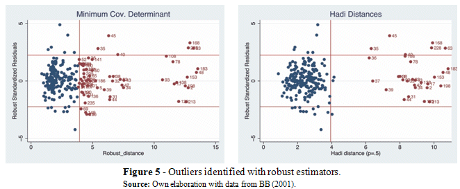
<body><![CDATA[<p align="center"><a name="t4"></a><img src="/img/revistas/riyd/v2n17/a02_table_04.gif" width="748" height="584"><font size="2" face="Verdana, Arial, Helvetica, sans-serif"><i>&nbsp;</i></font></p>      <p align="justify"><font size="2" face="Verdana, Arial, Helvetica, sans-serif">&#9679;&nbsp; <b>High breakdown point estimators</b></font></p>      <p align="justify"><font size="2" face="Verdana, Arial, Helvetica, sans-serif">We plot the Robust Standard Residuals in the <i>y</i>-axis versus robust Mahalanobis distances using MCD and Hadi distance methodologies, see     <a href="#f5">Figure 5</a>. The former gives an idea of the atypical data with respect to the fitted regression plane (on the <i>y</i>-axis), whereas the latter depicts the outlyingness of the explanatory variables (on the <i>x</i>-axis).</font></p>      <p align="justify"><font size="2" face="Verdana, Arial, Helvetica, sans-serif">The observations plotted in red are leverage points. For instance, country-pairs like Japan-Finland (45), Japan-France (35), Norway-Japan (168), Finland-Japan (228), and Denmark-Japan (63), among others are bad leverage points as they are outliers in the horizontal as well as in the vertical dimension. Contrarily, country-pairs such as Japan-Italy (37) or Japan-UK (39) are good leverage points since they are outlying in the horizontal dimension nor on the vertical one. As mentioned in Section 3 the presence of vertical outliers and bad leverage points might distort the coefficients and the standard errors of scrutiny.</font></p>      <p align="center"><a name="t5"></a><img src="/img/revistas/riyd/v2n17/a02_table_05.gif" width="745" height="648"></p>     <p align="center">&nbsp;</p>     <p align="center"><a name="f5"></a><img src="/img/revistas/riyd/v2n17/a02_figure_05.gif" width="662" height="273"></p>     <p align="justify"><font size="2" face="Verdana, Arial, Helvetica, sans-serif">To further explore the consequences of the presence of outliers, we compare the results of <a href="#t2">Table 2</a>, column (4) to the median regression (qreg) or L-estimator, Huber’s monotonic M-estimator (rreg), and the high breakdown MM-estimator (mmregress). <a href="#t6">Table 6</a> presents the results after a within transformation in the data. There are differences across methodologies, and as one can observe, the presence of outliers was biasing the results, in most cases, downwards. First, note that the coefficient estimate for income convergence (log(<i>s<sub>i</sub>s<sub>j</sub></i>)), it seems to be unimportant in explaining world trade growth (at a 10% level) when looking at the ordinary LS and median regression (columns (1) and (2)). However, when the influence of outliers and bad leverage points are taken into account (i.e., columns (4) and (5)), it turns out to be statistically significant different from zero at 1% level. Moreover, the coefficient estimate for the initial trade flow ( <img src="/img/revistas/riyd/v2n17/a02_e094.gif" width=87 height=14 align="absmiddle">) is no longer statistically significantly different from zero.</font></p>     <p align="center"><a name="t6"></a><img src="/img/revistas/riyd/v2n17/a02_table_06.gif" width="460" height="479"></p>     <p align="justify"><font size="2" face="Verdana, Arial, Helvetica, sans-serif">We study the regression threw by the MM-estimator due to its superior features. From Column (4), first, we confirm that transport-cost reduction explains 12 percentage points (or roughly 8%).<a href="#_ftn15" name="_ftnref15" title=""><sup><sup>[15]</sup></sup></a> Second, tariff-rate reduction explains 31 percentage points (or roughly 21%).<a href="#_ftn16" name="_ftnref16" title=""><sup><sup>[16]</sup></sup></a> That reveals an overestimation of the original results of seven percentage points. Third, we find that income convergence fall explains &#8722;2 percentage points (or roughly &#8722;2%).<a href="#_ftn17" name="_ftnref17" title=""><sup><sup>[17]</sup></sup></a> This coefficient is significant at 1% level. Last, bilateral income growth explains 104 percentage points, or the remainder, of this trade’s growth (71% of the total).<a href="#_ftn18" name="_ftnref18" title=""><sup><sup>[18]</sup></sup></a> Thus, under robust estimations income growth explains more of trade growth than previously stated, ten percentage points more.</font></p>     ]]></body>
<body><![CDATA[<p align="justify">&nbsp;</p>     <p align="justify"><font size="3" face="Verdana, Arial, Helvetica, sans-serif"><b>5. CONCLUSIONS</b></font><font size="2" face="Verdana, Arial, Helvetica, sans-serif"><b>&nbsp;</b></font></p>      <p align="justify"><font size="2" face="Verdana, Arial, Helvetica, sans-serif">This paper studies the robustness of BB (2001)’s seminal paper. The authors argue that ‘bilateral income growth explains about 67%, tariff-rate reductions about 25%, transport-cost declines about 8%, and income convergence represents virtually none of the average world trade growth.’ After briefly presenting BB (2001), we provide a step-by-step methodology for robustness checks in the presence of outliers in cross-sectional data analysis. We discuss classical methodologies for atypical points’ seeking such us, hat matrix, internally and externally standarized residuals, difference in fits, difference in betas, Cook’s distance, and Mahalanobis distance. Among the robust estimators utilized we the L-estimator, M-estimator, and MM-estimator, the latter being the most recommended.</font></p>      <p align="justify"><font size="2" face="Verdana, Arial, Helvetica, sans-serif">Overall, under MM estimation world trade can be attributed to 8% transport decreases, 21% to trade liberalization through tariffs reductions and 71% to income growth. Henceforth, even though BB (2001)’s results still hold, we conclude that under de presence of outliers trade liberalization has been overestimated in seven percentage points, while income growth has been underestimated by ten percentage points.</font></p>     <p align="justify"><font size="2" face="Verdana, Arial, Helvetica, sans-serif"><b>&nbsp;</b></font></p>     <p align="justify"><font size="3" face="Verdana, Arial, Helvetica, sans-serif"><b>6. ACKNOWLEDGMENTS</b></font><font size="2" face="Verdana, Arial, Helvetica, sans-serif"><b>&nbsp;</b></font></p>      <p align="justify"><font size="2" face="Verdana, Arial, Helvetica, sans-serif">We are particularly grateful to Scott Baier for helpful insights of his paper and also for kindly sharing his data set. We thank an anonymous referee for constructive comments, which contributed to improving the quality of the publication.</font></p>     <p align="justify">&nbsp;</p>     <p><font size="3"><b><font face="Verdana, Arial, Helvetica, sans-serif">NOTAS</font></b></font></p>     <p align="justify"><font size="2" face="Verdana, Arial, Helvetica, sans-serif"><a href="#_ftnref1" name="_ftn1" title=""><sup><sup>[1]</sup></sup></a> For formal theoretical foundations see   [20], [21], [22], [23], [24], and [25].</font></p>     ]]></body>
<body><![CDATA[<p align="justify"><font size="2" face="Verdana, Arial, Helvetica, sans-serif"><a href="#_ftnref2" name="_ftn2" title=""><sup><sup>[2]</sup></sup></a> In this paper we focus on the econometric part of the BB (2001)&rsquo;s paper,   rather than their theoretical contribution. This econometric approach has been   also used in [<a href="https://docs.google.com/document/d/19VQM_wWT6tc2FUNiGmidoKSMJTArJoE2GZJ_d3qWWG8/edit#bookmark=id.1ci93xb">26</a>].</font></p>     <p align="justify"><font size="2" face="Verdana, Arial, Helvetica, sans-serif"><a href="#_ftnref3" name="_ftn3" title=""><sup><sup>[3]</sup></sup></a> Provided that bilateral trade flow price deflators are not available, BB   (2001) use nominal trade flows adjusted for changes in the firms&rsquo;   price index: the exporter&rsquo;s GDP deflator.</font></p>     <p align="justify"><font size="2" face="Verdana, Arial, Helvetica, sans-serif"><a href="#_ftnref4" name="_ftn4" title=""><sup><sup>[4]</sup></sup></a> For example: <i>s<sub>i</sub></i> = <i>Y<sub>i</sub>/</i>(<i>Y<sub>i</sub></i> + <i>Y<sub>j</sub></i>)<i>.</i></font></p>     <p align="justify"><font size="2" face="Verdana, Arial, Helvetica, sans-serif"><a href="#_ftnref5" name="_ftn5" title=""><sup><sup>[5]</sup></sup></a> Income convergence is monotonically positively related to <i>s<sub>i</sub>s<sub>j</sub></i>,   which theoretically can vary from 0 to 0<i>.</i>25 (BB, 2001).</font></p>     <p align="justify"><font size="2" face="Verdana, Arial, Helvetica, sans-serif"><a href="#_ftnref6" name="_ftn6" title=""><sup><sup>[6]</sup></sup></a> This   is the outcome of simply dividing 23 percentage points by 147.63 percentage   points, taken from <a href="#t1">Table 1</a>.</font></p>     <p align="justify"><font size="2" face="Verdana, Arial, Helvetica, sans-serif"><a href="#_ftnref7" name="_ftn7" title=""><sup><sup>[7]</sup></sup></a> The contribution of 38 percentage points is reached from the product of   the mean logarithmic change of the tariff variable (-8.5 percentage points) and   its coefficient estimate (4.49).</font></p>     <p align="justify"><font size="2" face="Verdana, Arial, Helvetica, sans-serif"><a href="#_ftnref8" name="_ftn8" title=""><sup><sup>[8]</sup></sup></a> The contribution of 12 percentage points is achieved from the product of   the mean logarithmic change of the gross c.i.f.-f.o.b. factor (-3.6 percentage   points) and its coefficient estimate (3.19).</font></p>     <p align="justify"><font size="2" face="Verdana, Arial, Helvetica, sans-serif"><a href="#_ftnref9" name="_ftn9" title=""><sup><sup>[9]</sup></sup></a> This is obtained from four factors. First, the   product of the mean logarithmic of the bilateral income growth (105 percentage   points) and its coefficient estimate (2.37) yields 249 percentage   points. Second, the mean growth in importer income (103 percentage points)   times its coefficient (-0.68) yield -70 percentage points.   Third, the effect of the lagged trade flow (1108) times its   coefficient estimate (-0.08) yields -0.83 percentage points.   Forth, the product of GDP shares (-3.31 percentage points) times its coefficient   estimate (0.59) yields -2 percentage points. Adding the results yield   249-70-83-2=94 percentage points. The contribution of income growth in BB   (2001) is 100 percentage points after adding the constant, even though is not   significant.</font></p>     <p align="justify"><font size="2" face="Verdana, Arial, Helvetica, sans-serif"><a href="#_ftnref10" name="_ftn10" title=""><sup><sup>[10]</sup></sup></a> The hat matrix was introduced by   Tukey, John Wilder in 1972 [28].</font></p>     <p align="justify"><font size="2" face="Verdana, Arial, Helvetica, sans-serif"><a href="#_ftnref11" name="_ftn11" title=""><sup><sup>[11]</sup></sup></a>Named after the American   statistician R. Dennis Cook, who introduced the concept in [37, 38].</font></p>     ]]></body>
<body><![CDATA[<p align="justify"><font size="2" face="Verdana, Arial, Helvetica, sans-serif"><a href="#_ftnref12" name="_ftn12" title=""><sup><sup>[12]</sup></sup></a>Mahalanobis distances are   distributed as&nbsp;<img src="/img/revistas/riyd/v2n17/a02_e095.gif" width=17 height=14 align="bottom">&nbsp;for Gaussian data. Observe that <img src="/img/revistas/riyd/v2n17/a02_e096.gif" width=112 height=20 align="absmiddle">. Hence, <img src="/img/revistas/riyd/v2n17/a02_e097.gif" width=120 height=25 align="absmiddle">. For details of the proof see [32, p. 70]. </font></p>     <p align="justify"><font size="2" face="Verdana, Arial, Helvetica, sans-serif"><a href="#_ftnref13" name="_ftn13" title=""><sup><sup>[13]</sup></sup></a> Cases with Cook&rsquo;s distance greater than 1 are excluded   from the analysis.</font></p>     <p align="justify"><font size="2" face="Verdana, Arial, Helvetica, sans-serif"><a href="#_ftnref14" name="_ftn14" title=""><sup><sup>[14]</sup></sup></a> The constant is not significant even in the original   model. </font></p>     <p align="justify"><font size="2" face="Verdana, Arial, Helvetica, sans-serif"><a href="#_ftnref15" name="_ftn15" title=""><sup><sup>[15]</sup></sup></a> The contribution of 12 percentage points is   attained from the product of the mean logarithmic change of the gross c.i.f.-f.o.b.   factor (-3.6 percentage points) and its coefficient   estimate (-3.39).</font></p>     <p align="justify"><font size="2" face="Verdana, Arial, Helvetica, sans-serif"><a href="#_ftnref16" name="_ftn16" title=""><sup><sup>[16]</sup></sup></a> The contribution of 31 percentage points is   retrieved from the product of the mean logarithmic change of the tariff   variable (-8.5 percentage points) and its coefficient   estimate (-3.69).</font></p>     <p align="justify"><font size="2" face="Verdana, Arial, Helvetica, sans-serif"><a href="#_ftnref17" name="_ftn17" title=""><sup><sup>[17]</sup></sup></a>The contribution of &#8722;2 percentage points   is obtained from the product of the mean logarithmic change of the income   convergence variable (&#8722;3<i>.</i>3 percentage points) and its coefficient   estimate (0<i>.</i>75).</font></p>     <p align="justify"><font size="2" face="Verdana, Arial, Helvetica, sans-serif"><a href="#_ftnref18" name="_ftn18" title=""><sup><sup>[18]</sup></sup></a> This calculation is similar to the one   presented in footnote 9.</font></p>     <p align="justify">&nbsp;</p>     <p align="justify"><font size="3" face="Verdana, Arial, Helvetica, sans-serif"><b>7. REFERENCES</b></font><font size="2" face="Verdana, Arial, Helvetica, sans-serif"><b>&nbsp;</b></font></p>      <p align="justify"><font size="2" face="Verdana, Arial, Helvetica, sans-serif">[1]   S. L. Baier and J. H.   Bergstrand, &ldquo;The growth of world trade: tariffs, transport costs, and income   similarity,&rdquo; <i>Journal of International Economics</i>, vol. 53, pp. 1&ndash;27, 2001.</font></p>      ]]></body>
<body><![CDATA[<p align="justify"><font size="2" face="Verdana, Arial, Helvetica, sans-serif">[2]   P. Krugman, &ldquo;Growing world   trade: Causes and consequences.&rdquo; <i>Brookings Papers on</i> <i>Economic     Activity</i>, vol. 1, pp. 327&ndash;377, 1995.</font></p>     <p align="justify"><font size="2" face="Verdana, Arial, Helvetica, sans-serif">[3]   E. Helpman, &ldquo;Imperfect   competition and international trade: Evidence from fourteen industrial   countries,&rdquo; <i>Journal of the Japanese and International Economies</i>, vol. 1,   no. 1, pp. 62&ndash;81, 1987.</font></p>     <p align="justify"><font size="2" face="Verdana, Arial, Helvetica, sans-serif">[4]   D. Hummels and J. Levinsohn,   &ldquo;Monopolistic competition and international trade: Re-considering the   evidence,&rdquo; <i>Quarterly Journal of Economics</i>, vol. 110, no. 3, pp. 799&ndash;836,   1995.</font></p>     <!-- ref --><p align="justify"><font size="2" face="Verdana, Arial, Helvetica, sans-serif">[5]   J. Tinbergen, <i>Shaping     the World Economy: Suggestions for an International Economic</i> <i>Policy</i>.   The Twentieth Century Fund, New York, 1962.</font>&nbsp;&nbsp;&nbsp;&nbsp;&nbsp;&nbsp;&nbsp;&nbsp;[&#160;<a href="javascript:void(0);" onclick="javascript: window.open('/scielo.php?script=sci_nlinks&ref=965439&pid=S2518-4431201700020000200005&lng=','','width=640,height=500,resizable=yes,scrollbars=1,menubar=yes,');">Links</a>&#160;]<!-- end-ref --><p align="justify"><font size="2" face="Verdana, Arial, Helvetica, sans-serif">[6]   R. Baldwin, &ldquo;Towards an   integrated europe,&rdquo; <i>Centre for Economic Policy Research,</i> <i>London</i>,   1994.</font></p>     <p align="justify"><font size="2" face="Verdana, Arial, Helvetica, sans-serif">[7]   V. Oguledo and C. MacPhee,   &ldquo;Gravity models: A reformulation and an application to discriminatory trade   arrangements,&rdquo; <i>Applied Economics</i>, vol. 26, pp. 107&ndash;120, 1994.</font></p>     <p align="justify"><font size="2" face="Verdana, Arial, Helvetica, sans-serif">[8]   J. Frankel, &ldquo;Regional   trading blocs in the world economic system,&rdquo; <i>Institute for International     Economics, Washington, DC</i>, 1997.</font></p>     <p align="justify"><font size="2" face="Verdana, Arial, Helvetica, sans-serif">[9]   J. Wagner, &ldquo;International   trade and firm performance: a survey of empirical studies since 2006,&rdquo; <i>Review     of World Economics</i>, vol. 148, pp. 235&ndash;267, 2012.</font></p>     <!-- ref --><p align="justify"><font size="2" face="Verdana, Arial, Helvetica, sans-serif">[10]   P. J. Rousseeuw and A.   Leroy, Robust Regression and Outlier Detection. Wiley, New York, NY, 1987.</font>&nbsp;&nbsp;&nbsp;&nbsp;&nbsp;&nbsp;&nbsp;&nbsp;[&#160;<a href="javascript:void(0);" onclick="javascript: window.open('/scielo.php?script=sci_nlinks&ref=965444&pid=S2518-4431201700020000200010&lng=','','width=640,height=500,resizable=yes,scrollbars=1,menubar=yes,');">Links</a>&#160;]<!-- end-ref --><p align="justify"><font size="2" face="Verdana, Arial, Helvetica, sans-serif">[11]   C. Dehon, M. Gassner, and   V. Verardi, &ldquo;A Hausman-type test to detect the presence of influential outliers   in regression analysis,&rdquo; <i>Economic Letters</i>, pp. 64&ndash;67, 2009.</font></p>     ]]></body>
<body><![CDATA[<!-- ref --><p align="justify"><font size="2" face="Verdana, Arial, Helvetica, sans-serif">[12]   R. Maronna, D. Martin, and   V. Yohai, <i>Robust Statistics: Theory and Methods</i>. Wiley, New York, 2006.</font>&nbsp;&nbsp;&nbsp;&nbsp;&nbsp;&nbsp;&nbsp;&nbsp;[&#160;<a href="javascript:void(0);" onclick="javascript: window.open('/scielo.php?script=sci_nlinks&ref=965446&pid=S2518-4431201700020000200012&lng=','','width=640,height=500,resizable=yes,scrollbars=1,menubar=yes,');">Links</a>&#160;]<!-- end-ref --><p align="justify"><font size="2" face="Verdana, Arial, Helvetica, sans-serif">[13]   P. J. Rousseeuw and B. v.   Zomeren, &ldquo;Unmasking multivariate outliers and leverage points,&rdquo; <i>Journal of     the American Statistical Association</i>, vol. 85, pp. 633&ndash;639, 1990.</font></p>     <p align="justify"><font size="2" face="Verdana, Arial, Helvetica, sans-serif">[14]   J. Temple, &ldquo;Robustness   tests of the augmented Solow model,&rdquo; <i>Journal of Applied Econometrics</i>,   vol. 13, pp. 361&ndash;375, 1998.</font></p>     <p align="justify"><font size="2" face="Verdana, Arial, Helvetica, sans-serif">[15]   J. Temple, &ldquo;Growth   regressions and what the textbooks don&rsquo;t tell you,&rdquo; <i>Bulletin of</i> <i>Economic     Research</i>, vol. 52, pp. 181&ndash;205, 2000.</font></p>     <p align="justify"><font size="2" face="Verdana, Arial, Helvetica, sans-serif">[16]   D. Ruppert and D. G.   Simpson, &ldquo;Comment on Rousseeuw and van Zomeren,&rdquo; <i>Journal of</i> <i>the     American Statistical Association</i>, vol. 85, pp. 644&ndash;646, 1990.</font></p>     <p align="justify"><font size="2" face="Verdana, Arial, Helvetica, sans-serif">[17]   C. Croux, &ldquo;Are good   leverage points good or bad?,&rdquo; in <i>Paper Presented at the International     Conference on Robust Statistics</i>, 2006.</font></p>     <p align="justify"><font size="2" face="Verdana, Arial, Helvetica, sans-serif">[18]   C. Croux and C. Dehon,   &ldquo;Estimators of the multiple correlation coefficient: local robustness and   confidence intervals,&rdquo; <i>Statistical Papers</i>, vol. 44, pp. 315&ndash;334, 2003.</font></p>     <p align="justify"><font size="2" face="Verdana, Arial, Helvetica, sans-serif">[19]   B. Eichengreen and D.   Irwin, &ldquo;Trade blocs, currency blocs and the reorientation of world trade in the   1930s,&rdquo; <i>Journal of International Economics</i>, vol. 38 (1/2), pp. 1&ndash;24,   1995.</font></p>     <p align="justify"><font size="2" face="Verdana, Arial, Helvetica, sans-serif">[20]   J. Anderson, &ldquo;A theoretical   foundation for the gravity equation,&rdquo; <i>American Economic</i> <i>Review</i>,   vol. 69, no. 1, pp. 106&ndash;116, 1979.</font></p>     <p align="justify"><font size="2" face="Verdana, Arial, Helvetica, sans-serif">[21]   P. Krugman, &ldquo;Increasing   returns, monopolistic competition, and international trade,&rdquo; <i>Journal of     International Economics</i>, vol. 9, pp. 469&ndash;479, 1979.</font></p>     ]]></body>
<body><![CDATA[<!-- ref --><p align="justify"><font size="2" face="Verdana, Arial, Helvetica, sans-serif">[22]   E. Helpman and P. Krugman, <i>Market Structure and Foreign Trade</i>. MIT Press, Cambridge, MA, 1985.</font>&nbsp;&nbsp;&nbsp;&nbsp;&nbsp;&nbsp;&nbsp;&nbsp;[&#160;<a href="javascript:void(0);" onclick="javascript: window.open('/scielo.php?script=sci_nlinks&ref=965456&pid=S2518-4431201700020000200022&lng=','','width=640,height=500,resizable=yes,scrollbars=1,menubar=yes,');">Links</a>&#160;]<!-- end-ref --><p align="justify"><font size="2" face="Verdana, Arial, Helvetica, sans-serif">[23]   J. H. Bergstrand, &ldquo;The   gravity equation in international trade: Some microeconomic foundations and   empirical evidence,&rdquo; <i>Review of Economics and Statistics</i>, vol. 67 (3),   474&ndash;481, 1985.</font></p>     <p align="justify"><font size="2" face="Verdana, Arial, Helvetica, sans-serif">[24]   J. H. Bergstrand, &ldquo;The   generalized gravity equation, monopolistic competition, and the   factor-proportions theory in international trade,&rdquo; <i>Review of Economics and     Statistics</i>, vol. 71 (1), pp. 143&ndash;153, 1989.</font></p>     <p align="justify"><font size="2" face="Verdana, Arial, Helvetica, sans-serif">[25]   J. H. Bergstrand, &ldquo;The Heckscher-Ohlin-Samuelson   model, the linder hypothesis, and the determinants of bilateral intra-industry   trade,&rdquo; <i>Economic Journal</i>, vol. 100 (4), 1216&ndash;1229, 1990.</font></p>     <p align="justify"><font size="2" face="Verdana, Arial, Helvetica, sans-serif">[26]   T. Bayoumi and B.   Eichengreen, <i>Regionalism versus Multilateral Trade Arrangements</i>, ch. Is   regionalism simply a diversion? Evidence from the EU and EFTA. The University   of Chicago Press, Chicago, 1997.</font></p>     <p align="justify"><font size="2" face="Verdana, Arial, Helvetica, sans-serif">[27]   P. Krugman, &ldquo;Scale   economies, product differentiation, and the pattern of trade,&rdquo; <i>American     Economic Review</i>, vol. 70, no. 5, pp. 950&ndash;959, 1980.</font></p>     <p align="justify"><font size="2" face="Verdana, Arial, Helvetica, sans-serif">[28]   D. C. Hoaglin and R. E.   Welsch, &ldquo;The hat matrix in regression and anova,&rdquo; <i>The American</i> <i>Statistician</i>,   vol. 32, no. 1, pp. 17&ndash;22, 1978.</font></p>     <p align="justify"><font size="2" face="Verdana, Arial, Helvetica, sans-serif">[29]   B. W. Silverman, &ldquo;Spline   smoothing: The equivalent variable kernel method,&rdquo; <i>The</i> <i>Annals of     Statistics</i>, vol. 12, no. 3, pp. 898&ndash;916, 1984.</font></p>     <p align="justify"><font size="2" face="Verdana, Arial, Helvetica, sans-serif">[30]   R. Eubank, &ldquo;The hat matrix   for smoothing splines,&rdquo; <i>Statistics and Probability Letters</i>, vol. 2, no.   1, pp. 9&ndash;14, 1984.</font></p>     <p align="justify"><font size="2" face="Verdana, Arial, Helvetica, sans-serif">[31]   J. Li and R. Valliant,   &ldquo;Survey weighted hat matrix and leverages,&rdquo; <i>Survey Methodology</i>, vol. 35,   no. 1, pp. 15&ndash;24, 2009.</font></p>     ]]></body>
<body><![CDATA[<!-- ref --><p align="justify"><font size="2" face="Verdana, Arial, Helvetica, sans-serif">[32]   V. Verardi, <i>Robust     Regression in Stata</i>. FUNDP (Namur) and ULB (Brussels), Belgium, 2009.</font>&nbsp;&nbsp;&nbsp;&nbsp;&nbsp;&nbsp;&nbsp;&nbsp;[&#160;<a href="javascript:void(0);" onclick="javascript: window.open('/scielo.php?script=sci_nlinks&ref=965466&pid=S2518-4431201700020000200032&lng=','','width=640,height=500,resizable=yes,scrollbars=1,menubar=yes,');">Links</a>&#160;]<!-- end-ref --><p align="justify"><font size="2" face="Verdana, Arial, Helvetica, sans-serif">[33]   S. Chatterjee and A. S.   Hadi, &ldquo;Influential observations, high leveraleverage, and outliers in linear   regression,&rdquo; <i>Statistical Science</i>, vol. 1, no. 3, pp. 379&ndash;416, 1986.</font></p>     <p align="justify"><font size="2" face="Verdana, Arial, Helvetica, sans-serif">[34]   V. Verardi and C. Croux,   &ldquo;Robust regression in Stata,&rdquo; <i>The Stata Journal</i>, vol. 9, 439&ndash;453, 2009.</font></p>     <!-- ref --><p align="justify"><font size="2" face="Verdana, Arial, Helvetica, sans-serif">[35]   D. C. Montgomery and E. A.   Peck, <i>Introduction to linear regression analysis</i>. Wiley, 1982.</font>&nbsp;&nbsp;&nbsp;&nbsp;&nbsp;&nbsp;&nbsp;&nbsp;[&#160;<a href="javascript:void(0);" onclick="javascript: window.open('/scielo.php?script=sci_nlinks&ref=965469&pid=S2518-4431201700020000200035&lng=','','width=640,height=500,resizable=yes,scrollbars=1,menubar=yes,');">Links</a>&#160;]<!-- end-ref --><p align="justify"><font size="2" face="Verdana, Arial, Helvetica, sans-serif">[36]   J. B. Gray and W. H.   Woodall, &ldquo;The maximum size of standardized and internally studentized residuals   in regression analysis,&rdquo; <i>The American Statistician</i>, vol. 48, no. 2,   111&ndash;113, 1994.</font></p>     <p align="justify"><font size="2" face="Verdana, Arial, Helvetica, sans-serif">[37]   R. D. Cook, &ldquo;Detection of   influential observations in linear regression,&rdquo; <i>Technometrics.</i> <i>American     Statistical Association</i>, vol. 19, no. 1, pp. 15&ndash;18, 1977.</font></p>     <p align="justify"><font size="2" face="Verdana, Arial, Helvetica, sans-serif">[38]   R. D. Cook, &ldquo;Influential   observations in linear regression,&rdquo; <i>Journal of the American</i> <i>Statistical     Association. American Statistical Association</i>, vol. 74, no. 365, pp.   169&ndash;174, 1979.</font></p>     <!-- ref --><p align="justify"><font size="2" face="Verdana, Arial, Helvetica, sans-serif">[39]   R. D. Cook and S.   Weisberg, <i>Residuals and Influence in Regression</i>. New York, NY, 1982.</font>&nbsp;&nbsp;&nbsp;&nbsp;&nbsp;&nbsp;&nbsp;&nbsp;[&#160;<a href="javascript:void(0);" onclick="javascript: window.open('/scielo.php?script=sci_nlinks&ref=965473&pid=S2518-4431201700020000200039&lng=','','width=640,height=500,resizable=yes,scrollbars=1,menubar=yes,');">Links</a>&#160;]<!-- end-ref --><p align="justify"><font size="2" face="Verdana, Arial, Helvetica, sans-serif">[40]   K. A. Bollen and R. W.   Jackman, <i>Modern Methods of Data Analysis</i>, ch. Regression Diagnostics: An   Expository Treatment of Outliers and Influential Cases, pp. 257&ndash;291. Newbury   Park, CA: Sage press, 1990.</font></p>     <p align="justify"><font size="2" face="Verdana, Arial, Helvetica, sans-serif">[41]   P. C. Mahalanobis, &ldquo;On the   generalised distance in statistics,&rdquo; <i>Proceedings of the National Institute     of Sciences of India</i>, vol. 2, no. 1, pp. 49&ndash;55, 1936.</font></p>     ]]></body>
<body><![CDATA[<p align="justify"><font size="2" face="Verdana, Arial, Helvetica, sans-serif">[42]   K. I. Penny, &ldquo;Appropriate   critical values when testing for a single multivariate outlier by using the   mahalanobis distance,&rdquo; <i>Journal of the Royal Statistical Society</i>, vol.   45, no. 1, 73&ndash;81, 1996.</font></p>     <p align="justify"><font size="2" face="Verdana, Arial, Helvetica, sans-serif">[43]   V. Verardi and A.   McCathie, &ldquo;The s-estimator of multivariate location and scatter in stata,&rdquo; <i>Stata     Journal, StataCorp LP</i>, vol. 12, pp. 299&ndash;307, June 2012.</font></p>     <p align="justify"><font size="2" face="Verdana, Arial, Helvetica, sans-serif">[44]   V. Verardi and C. Dehon,   &ldquo;Multivariate outlier detection in stata,&rdquo; <i>Stata Journal, StataCorp</i>,   vol. 10, no. 2, pp. 259&ndash;266, 2010.</font></p>     <p align="justify"><font size="2" face="Verdana, Arial, Helvetica, sans-serif">[45]   S. S. Wilks, &ldquo;Certain   generalizations in the analysis of variance,&rdquo; <i>Biometrika</i>, vol. 24,   471&ndash;494, 1932.</font></p>     <p align="justify"><font size="2" face="Verdana, Arial, Helvetica, sans-serif">[46]   A. S. Hadi, &ldquo;Identifying   multiple outliers in multivariate data,&rdquo; <i>Journal of the Royal</i> <i>Statistical     Society</i>, pp. 761&ndash;771, 1992.</font></p>     <p align="justify"><font size="2" face="Verdana, Arial, Helvetica, sans-serif">[47]   P. J. Huber, &ldquo;Robust   estimation of a location parameter,&rdquo; <i>The Annals of Mathematical</i> <i>Statistics</i>,   vol. 35, no. 1, pp. 73&ndash;101, 1964.</font></p> <hr align=JUSTIFY size=1 width="33%">      ]]></body><back>
<ref-list>
<ref id="B1">
<label>1</label><nlm-citation citation-type="journal">
<person-group person-group-type="author">
<name>
<surname><![CDATA[Baier]]></surname>
<given-names><![CDATA[S.L.]]></given-names>
</name>
<name>
<surname><![CDATA[Bergstrand]]></surname>
<given-names><![CDATA[J.H.]]></given-names>
</name>
</person-group>
<article-title xml:lang="en"><![CDATA[The growth of world trade: tariffs, transport costs%cc and income similarity]]></article-title>
<source><![CDATA[Journal of International Economics]]></source>
<year>2001</year>
<volume>53</volume>
<page-range>1-27</page-range></nlm-citation>
</ref>
<ref id="B2">
<label>2</label><nlm-citation citation-type="journal">
<person-group person-group-type="author">
<name>
<surname><![CDATA[Krugman]]></surname>
<given-names><![CDATA[P.]]></given-names>
</name>
</person-group>
<article-title xml:lang="en"><![CDATA[Growing world trade: Causes and consequences]]></article-title>
<source><![CDATA[Brookings Papers on Economic Activity]]></source>
<year>1995</year>
<volume>1</volume>
<page-range>327-377</page-range></nlm-citation>
</ref>
<ref id="B3">
<label>3</label><nlm-citation citation-type="journal">
<person-group person-group-type="author">
<name>
<surname><![CDATA[Helpman]]></surname>
<given-names><![CDATA[E.]]></given-names>
</name>
</person-group>
<article-title xml:lang="en"><![CDATA[Imperfect competition and international trade: Evidence from fourteen industrial countries]]></article-title>
<source><![CDATA[Journal of the Japanese and International Economies]]></source>
<year>1987</year>
<volume>1</volume>
<numero>1</numero>
<issue>1</issue>
<page-range>62-81</page-range></nlm-citation>
</ref>
<ref id="B4">
<label>4</label><nlm-citation citation-type="journal">
<person-group person-group-type="author">
<name>
<surname><![CDATA[Hummels]]></surname>
<given-names><![CDATA[D.]]></given-names>
</name>
<name>
<surname><![CDATA[Levinsohn]]></surname>
<given-names><![CDATA[J.]]></given-names>
</name>
</person-group>
<article-title xml:lang="en"><![CDATA[Monopolistic competition and international trade: Re-considering the evidence]]></article-title>
<source><![CDATA[Quarterly Journal of Economics]]></source>
<year>1995</year>
<volume>110</volume>
<numero>3</numero>
<issue>3</issue>
<page-range>799-836</page-range></nlm-citation>
</ref>
<ref id="B5">
<label>5</label><nlm-citation citation-type="book">
<person-group person-group-type="author">
<name>
<surname><![CDATA[Tinbergen]]></surname>
<given-names><![CDATA[J.]]></given-names>
</name>
</person-group>
<source><![CDATA[Shaping the World Economy: Suggestions for an International Economic Policy]]></source>
<year>1962</year>
<publisher-loc><![CDATA[New York ]]></publisher-loc>
<publisher-name><![CDATA[The Twentieth Century Fund]]></publisher-name>
</nlm-citation>
</ref>
<ref id="B6">
<label>6</label><nlm-citation citation-type="book">
<person-group person-group-type="author">
<name>
<surname><![CDATA[Baldwin]]></surname>
<given-names><![CDATA[R.]]></given-names>
</name>
</person-group>
<source><![CDATA[Towards an integrated Europe]]></source>
<year>1994</year>
<publisher-loc><![CDATA[London ]]></publisher-loc>
<publisher-name><![CDATA[Centre for Economic Policy Research]]></publisher-name>
</nlm-citation>
</ref>
<ref id="B7">
<label>7</label><nlm-citation citation-type="journal">
<person-group person-group-type="author">
<name>
<surname><![CDATA[Oguledo]]></surname>
<given-names><![CDATA[V.]]></given-names>
</name>
<name>
<surname><![CDATA[MacPhee]]></surname>
<given-names><![CDATA[C.]]></given-names>
</name>
</person-group>
<article-title xml:lang="en"><![CDATA[Gravity models: A reformulation and an application to discriminatory trade arrangements]]></article-title>
<source><![CDATA[Applied Economics]]></source>
<year>1994</year>
<volume>26</volume>
<page-range>107-120</page-range></nlm-citation>
</ref>
<ref id="B8">
<label>8</label><nlm-citation citation-type="book">
<person-group person-group-type="author">
<name>
<surname><![CDATA[Frankel]]></surname>
<given-names><![CDATA[J.]]></given-names>
</name>
</person-group>
<source><![CDATA[Regional trading blocs in the world economic system]]></source>
<year>1997</year>
<publisher-loc><![CDATA[Washington^eDC DC]]></publisher-loc>
<publisher-name><![CDATA[Institute for International Economics]]></publisher-name>
</nlm-citation>
</ref>
<ref id="B9">
<label>9</label><nlm-citation citation-type="journal">
<person-group person-group-type="author">
<name>
<surname><![CDATA[Wagner]]></surname>
<given-names><![CDATA[J.]]></given-names>
</name>
</person-group>
<article-title xml:lang="en"><![CDATA[International trade and firm performance: a survey of empirical studies since 2006]]></article-title>
<source><![CDATA[Review of World Economics]]></source>
<year>2012</year>
<volume>148</volume>
<page-range>235-267</page-range></nlm-citation>
</ref>
<ref id="B10">
<label>10</label><nlm-citation citation-type="book">
<person-group person-group-type="author">
<name>
<surname><![CDATA[Rousseeuw]]></surname>
<given-names><![CDATA[P.J.]]></given-names>
</name>
<name>
<surname><![CDATA[Leroy]]></surname>
<given-names><![CDATA[A.]]></given-names>
</name>
</person-group>
<source><![CDATA[Robust Regression and Outlier Detection]]></source>
<year>1987</year>
<publisher-loc><![CDATA[New York^eNY NY]]></publisher-loc>
<publisher-name><![CDATA[Wiley]]></publisher-name>
</nlm-citation>
</ref>
<ref id="B11">
<label>11</label><nlm-citation citation-type="journal">
<person-group person-group-type="author">
<name>
<surname><![CDATA[Dehon]]></surname>
<given-names><![CDATA[C.]]></given-names>
</name>
<name>
<surname><![CDATA[Gassner]]></surname>
<given-names><![CDATA[M.]]></given-names>
</name>
<name>
<surname><![CDATA[Verardi]]></surname>
<given-names><![CDATA[V.]]></given-names>
</name>
</person-group>
<article-title xml:lang="en"><![CDATA[A Hausman-type test to detect the presence of influential outliers in regression analysis]]></article-title>
<source><![CDATA[Economic Letters]]></source>
<year>2009</year>
<page-range>64-67</page-range></nlm-citation>
</ref>
<ref id="B12">
<label>12</label><nlm-citation citation-type="book">
<person-group person-group-type="author">
<name>
<surname><![CDATA[Maronna]]></surname>
<given-names><![CDATA[R.]]></given-names>
</name>
<name>
<surname><![CDATA[Martin]]></surname>
<given-names><![CDATA[D.]]></given-names>
</name>
<name>
<surname><![CDATA[Yohai]]></surname>
<given-names><![CDATA[V.]]></given-names>
</name>
</person-group>
<source><![CDATA[Robust Statistics: Theory and Methods]]></source>
<year>2006</year>
<publisher-loc><![CDATA[New York ]]></publisher-loc>
<publisher-name><![CDATA[Wiley]]></publisher-name>
</nlm-citation>
</ref>
<ref id="B13">
<label>13</label><nlm-citation citation-type="journal">
<person-group person-group-type="author">
<name>
<surname><![CDATA[Rousseeuw]]></surname>
<given-names><![CDATA[P.J.]]></given-names>
</name>
<name>
<surname><![CDATA[Zomeren]]></surname>
<given-names><![CDATA[B.V.]]></given-names>
</name>
</person-group>
<article-title xml:lang="en"><![CDATA[Unmasking multivariate outliers and leverage points]]></article-title>
<source><![CDATA[Journal of the American Statistical Association]]></source>
<year>1990</year>
<volume>85</volume>
<page-range>633-639</page-range></nlm-citation>
</ref>
<ref id="B14">
<label>14</label><nlm-citation citation-type="journal">
<person-group person-group-type="author">
<name>
<surname><![CDATA[Temple]]></surname>
<given-names><![CDATA[J.]]></given-names>
</name>
</person-group>
<article-title xml:lang="en"><![CDATA[Robustness tests of the augmented Solow model]]></article-title>
<source><![CDATA[Journal of Applied Econometrics]]></source>
<year>1998</year>
<volume>13</volume>
<page-range>361-375</page-range></nlm-citation>
</ref>
<ref id="B15">
<label>15</label><nlm-citation citation-type="journal">
<person-group person-group-type="author">
<name>
<surname><![CDATA[Temple]]></surname>
<given-names><![CDATA[J.]]></given-names>
</name>
</person-group>
<article-title xml:lang="en"><![CDATA[Growth regressions and what the textbooks don’t tell you]]></article-title>
<source><![CDATA[Bulletin of Economic Research]]></source>
<year>2000</year>
<volume>52</volume>
<page-range>181-205</page-range></nlm-citation>
</ref>
<ref id="B16">
<label>16</label><nlm-citation citation-type="journal">
<person-group person-group-type="author">
<name>
<surname><![CDATA[Ruppert]]></surname>
<given-names><![CDATA[D.]]></given-names>
</name>
<name>
<surname><![CDATA[Simpson]]></surname>
<given-names><![CDATA[D.G.]]></given-names>
</name>
</person-group>
<article-title xml:lang="en"><![CDATA[Comment on Rousseeuw and van Zomeren]]></article-title>
<source><![CDATA[Journal of the American Statistical Association]]></source>
<year>1990</year>
<volume>85</volume>
<page-range>644-646</page-range></nlm-citation>
</ref>
<ref id="B17">
<label>17</label><nlm-citation citation-type="confpro">
<person-group person-group-type="author">
<name>
<surname><![CDATA[Croux]]></surname>
<given-names><![CDATA[C.]]></given-names>
</name>
</person-group>
<source><![CDATA[Are good leverage points good or bad?]]></source>
<year>2006</year>
<conf-name><![CDATA[ International Conference on Robust Statistics]]></conf-name>
<conf-loc> </conf-loc>
</nlm-citation>
</ref>
<ref id="B18">
<label>18</label><nlm-citation citation-type="journal">
<person-group person-group-type="author">
<name>
<surname><![CDATA[Croux]]></surname>
<given-names><![CDATA[C.]]></given-names>
</name>
<name>
<surname><![CDATA[Dehon]]></surname>
<given-names><![CDATA[C.]]></given-names>
</name>
</person-group>
<article-title xml:lang="en"><![CDATA[Estimators of the multiple correlation coefficient: local robustness and confidence intervals]]></article-title>
<source><![CDATA[Statistical Papers]]></source>
<year>2003</year>
<volume>44</volume>
<page-range>315-334</page-range></nlm-citation>
</ref>
<ref id="B19">
<label>19</label><nlm-citation citation-type="journal">
<person-group person-group-type="author">
<name>
<surname><![CDATA[Eichengreen]]></surname>
<given-names><![CDATA[B.]]></given-names>
</name>
<name>
<surname><![CDATA[Irwin]]></surname>
<given-names><![CDATA[D.]]></given-names>
</name>
</person-group>
<article-title xml:lang="en"><![CDATA[Trade blocs, currency blocs and the reorientation of world trade in the 1930s]]></article-title>
<source><![CDATA[Journal of International Economics]]></source>
<year>1995</year>
<volume>38</volume>
<numero>1/2</numero>
<issue>1/2</issue>
<page-range>1-24</page-range></nlm-citation>
</ref>
<ref id="B20">
<label>20</label><nlm-citation citation-type="journal">
<person-group person-group-type="author">
<name>
<surname><![CDATA[Anderson]]></surname>
<given-names><![CDATA[J.]]></given-names>
</name>
</person-group>
<article-title xml:lang="en"><![CDATA[A theoretical foundation for the gravity equation]]></article-title>
<source><![CDATA[American Economic Review]]></source>
<year>1979</year>
<volume>69</volume>
<numero>1</numero>
<issue>1</issue>
<page-range>106-116</page-range></nlm-citation>
</ref>
<ref id="B21">
<label>21</label><nlm-citation citation-type="journal">
<person-group person-group-type="author">
<name>
<surname><![CDATA[Krugman]]></surname>
<given-names><![CDATA[P.]]></given-names>
</name>
</person-group>
<article-title xml:lang="en"><![CDATA[Increasing returns, monopolistic competition, and international trade]]></article-title>
<source><![CDATA[Journal of International Economics]]></source>
<year>1979</year>
<volume>9</volume>
<page-range>469-479</page-range></nlm-citation>
</ref>
<ref id="B22">
<label>22</label><nlm-citation citation-type="book">
<person-group person-group-type="author">
<name>
<surname><![CDATA[Helpman]]></surname>
<given-names><![CDATA[E.]]></given-names>
</name>
<name>
<surname><![CDATA[Krugman]]></surname>
<given-names><![CDATA[P.]]></given-names>
</name>
</person-group>
<source><![CDATA[Market Structure and Foreign Trade]]></source>
<year>1985</year>
<publisher-loc><![CDATA[Cambridge^eMA MA]]></publisher-loc>
<publisher-name><![CDATA[MIT Press]]></publisher-name>
</nlm-citation>
</ref>
<ref id="B23">
<label>23</label><nlm-citation citation-type="journal">
<person-group person-group-type="author">
<name>
<surname><![CDATA[Bergstrand]]></surname>
<given-names><![CDATA[J.H.]]></given-names>
</name>
</person-group>
<article-title xml:lang="en"><![CDATA[The gravity equation in international trade: Some microeconomic foundations and empirical evidence]]></article-title>
<source><![CDATA[Review of Economics and Statistics]]></source>
<year>1985</year>
<volume>67</volume>
<numero>3</numero>
<issue>3</issue>
<page-range>474-481</page-range></nlm-citation>
</ref>
<ref id="B24">
<label>24</label><nlm-citation citation-type="journal">
<person-group person-group-type="author">
<name>
<surname><![CDATA[Bergstrand]]></surname>
<given-names><![CDATA[J.H.]]></given-names>
</name>
</person-group>
<article-title xml:lang="en"><![CDATA[The generalized gravity equation, monopolistic competition, and the factor-proportions theory in international trade]]></article-title>
<source><![CDATA[Review of Economics and Statistics]]></source>
<year>1989</year>
<volume>71</volume>
<numero>1</numero>
<issue>1</issue>
<page-range>143-153</page-range></nlm-citation>
</ref>
<ref id="B25">
<label>25</label><nlm-citation citation-type="journal">
<person-group person-group-type="author">
<name>
<surname><![CDATA[Bergstrand]]></surname>
<given-names><![CDATA[J.H.]]></given-names>
</name>
</person-group>
<article-title xml:lang="en"><![CDATA[The Heckscher-Ohlin-Samuelson model, the linder hypothesis, and the determinants of bilateral intra-industry trade]]></article-title>
<source><![CDATA[Economic Journal]]></source>
<year>1990</year>
<volume>100</volume>
<numero>4</numero>
<issue>4</issue>
<page-range>1216-1229</page-range></nlm-citation>
</ref>
<ref id="B26">
<label>26</label><nlm-citation citation-type="book">
<person-group person-group-type="author">
<name>
<surname><![CDATA[Bayoumi]]></surname>
<given-names><![CDATA[T.]]></given-names>
</name>
<name>
<surname><![CDATA[Eichengreen]]></surname>
<given-names><![CDATA[B.]]></given-names>
</name>
</person-group>
<source><![CDATA[Regionalism versus Multilateral Trade Arrangements, Is regionalism simply a diversion? Evidence from the EU and EFTA]]></source>
<year>1997</year>
<publisher-loc><![CDATA[Chicago ]]></publisher-loc>
<publisher-name><![CDATA[The University of Chicago Press]]></publisher-name>
</nlm-citation>
</ref>
<ref id="B27">
<label>27</label><nlm-citation citation-type="journal">
<person-group person-group-type="author">
<name>
<surname><![CDATA[Krugman]]></surname>
<given-names><![CDATA[P.]]></given-names>
</name>
</person-group>
<article-title xml:lang="en"><![CDATA[Scale economies, product differentiation, and the pattern of trade]]></article-title>
<source><![CDATA[American Economic Review]]></source>
<year>1980</year>
<volume>70</volume>
<numero>5</numero>
<issue>5</issue>
<page-range>950-959</page-range></nlm-citation>
</ref>
<ref id="B28">
<label>28</label><nlm-citation citation-type="journal">
<person-group person-group-type="author">
<name>
<surname><![CDATA[Hoaglin]]></surname>
<given-names><![CDATA[D.C.]]></given-names>
</name>
<name>
<surname><![CDATA[Welsch]]></surname>
<given-names><![CDATA[R.E.]]></given-names>
</name>
</person-group>
<article-title xml:lang="en"><![CDATA[The hat matrix in regression and anova]]></article-title>
<source><![CDATA[The American Statistician]]></source>
<year>1978</year>
<volume>32</volume>
<numero>1</numero>
<issue>1</issue>
<page-range>17-22</page-range></nlm-citation>
</ref>
<ref id="B29">
<label>29</label><nlm-citation citation-type="journal">
<person-group person-group-type="author">
<name>
<surname><![CDATA[Silverman]]></surname>
<given-names><![CDATA[B.W.]]></given-names>
</name>
</person-group>
<article-title xml:lang="en"><![CDATA[Spline smoothing: The equivalent variable kernel method]]></article-title>
<source><![CDATA[The Annals of Statistics]]></source>
<year>1984</year>
<volume>12</volume>
<numero>3</numero>
<issue>3</issue>
<page-range>898-916</page-range></nlm-citation>
</ref>
<ref id="B30">
<label>30</label><nlm-citation citation-type="journal">
<person-group person-group-type="author">
<name>
<surname><![CDATA[Eubank]]></surname>
<given-names><![CDATA[R.]]></given-names>
</name>
</person-group>
<article-title xml:lang="en"><![CDATA[The hat matrix for smoothing splines]]></article-title>
<source><![CDATA[Statistics and Probability Letters]]></source>
<year>1984</year>
<volume>2</volume>
<numero>1</numero>
<issue>1</issue>
<page-range>9-14</page-range></nlm-citation>
</ref>
<ref id="B31">
<label>31</label><nlm-citation citation-type="journal">
<person-group person-group-type="author">
<name>
<surname><![CDATA[Li]]></surname>
<given-names><![CDATA[J.]]></given-names>
</name>
<name>
<surname><![CDATA[Valliant]]></surname>
<given-names><![CDATA[R.]]></given-names>
</name>
</person-group>
<article-title xml:lang="en"><![CDATA[Survey weighted hat matrix and leverages]]></article-title>
<source><![CDATA[Survey Methodology]]></source>
<year>2009</year>
<volume>35</volume>
<numero>1</numero>
<issue>1</issue>
<page-range>15-24</page-range></nlm-citation>
</ref>
<ref id="B32">
<label>32</label><nlm-citation citation-type="book">
<person-group person-group-type="author">
<name>
<surname><![CDATA[Verardi]]></surname>
<given-names><![CDATA[V.]]></given-names>
</name>
</person-group>
<source><![CDATA[Robust Regression in Stata]]></source>
<year>2009</year>
<publisher-loc><![CDATA[Belgium ]]></publisher-loc>
<publisher-name><![CDATA[FUNDP (Namur) and ULB (Brussels)]]></publisher-name>
</nlm-citation>
</ref>
<ref id="B33">
<label>33</label><nlm-citation citation-type="journal">
<person-group person-group-type="author">
<name>
<surname><![CDATA[Chatterjee]]></surname>
<given-names><![CDATA[S.]]></given-names>
</name>
<name>
<surname><![CDATA[Hadi]]></surname>
<given-names><![CDATA[A.S.]]></given-names>
</name>
</person-group>
<article-title xml:lang="en"><![CDATA[Influential observations, high leveraleverage, and outliers in linear regression]]></article-title>
<source><![CDATA[Statistical Science]]></source>
<year>1986</year>
<volume>1</volume>
<numero>3</numero>
<issue>3</issue>
<page-range>379-416</page-range></nlm-citation>
</ref>
<ref id="B34">
<label>34</label><nlm-citation citation-type="journal">
<person-group person-group-type="author">
<name>
<surname><![CDATA[Verardi]]></surname>
<given-names><![CDATA[V.]]></given-names>
</name>
<name>
<surname><![CDATA[Croux]]></surname>
<given-names><![CDATA[C.]]></given-names>
</name>
</person-group>
<article-title xml:lang="en"><![CDATA[Robust regression in Stata]]></article-title>
<source><![CDATA[The Stata Journal]]></source>
<year>2009</year>
<volume>9</volume>
<page-range>439-453</page-range></nlm-citation>
</ref>
<ref id="B35">
<label>35</label><nlm-citation citation-type="book">
<person-group person-group-type="author">
<name>
<surname><![CDATA[Montgomery]]></surname>
<given-names><![CDATA[D.C.]]></given-names>
</name>
<name>
<surname><![CDATA[Peck]]></surname>
<given-names><![CDATA[E.A.]]></given-names>
</name>
</person-group>
<source><![CDATA[Introduction to linear regression analysis]]></source>
<year>1982</year>
<publisher-name><![CDATA[Wiley]]></publisher-name>
</nlm-citation>
</ref>
<ref id="B36">
<label>36</label><nlm-citation citation-type="journal">
<person-group person-group-type="author">
<name>
<surname><![CDATA[Gray]]></surname>
<given-names><![CDATA[J.B.]]></given-names>
</name>
<name>
<surname><![CDATA[Woodall]]></surname>
<given-names><![CDATA[W.H.]]></given-names>
</name>
</person-group>
<article-title xml:lang="en"><![CDATA[The maximum size of standardized and internally studentized residuals in regression analysis]]></article-title>
<source><![CDATA[The American Statistician]]></source>
<year>1994</year>
<volume>48</volume>
<numero>2</numero>
<issue>2</issue>
<page-range>111-113</page-range></nlm-citation>
</ref>
<ref id="B37">
<label>37</label><nlm-citation citation-type="journal">
<person-group person-group-type="author">
<name>
<surname><![CDATA[Cook]]></surname>
<given-names><![CDATA[R.D.]]></given-names>
</name>
</person-group>
<article-title xml:lang="en"><![CDATA[Detection of influential observations in linear regression]]></article-title>
<source><![CDATA[Technometrics. American Statistical Association]]></source>
<year>1977</year>
<volume>19</volume>
<numero>1</numero>
<issue>1</issue>
<page-range>15-18</page-range></nlm-citation>
</ref>
<ref id="B38">
<label>38</label><nlm-citation citation-type="journal">
<person-group person-group-type="author">
<name>
<surname><![CDATA[Cook]]></surname>
<given-names><![CDATA[R.D.]]></given-names>
</name>
</person-group>
<article-title xml:lang="en"><![CDATA[Influential observations in linear regression]]></article-title>
<source><![CDATA[Journal of the American Statistical Association]]></source>
<year>1979</year>
<volume>74</volume>
<numero>365</numero>
<issue>365</issue>
<page-range>169-174</page-range><publisher-name><![CDATA[American Statistical Association]]></publisher-name>
</nlm-citation>
</ref>
<ref id="B39">
<label>39</label><nlm-citation citation-type="">
<person-group person-group-type="author">
<name>
<surname><![CDATA[D. Cook]]></surname>
<given-names><![CDATA[R.]]></given-names>
</name>
<name>
<surname><![CDATA[Weisberg]]></surname>
<given-names><![CDATA[S.]]></given-names>
</name>
</person-group>
<source><![CDATA[Residuals and Influence in Regression]]></source>
<year>1982</year>
<publisher-loc><![CDATA[New York^eNY NY]]></publisher-loc>
</nlm-citation>
</ref>
<ref id="B40">
<label>40</label><nlm-citation citation-type="book">
<person-group person-group-type="author">
<name>
<surname><![CDATA[Bollen]]></surname>
<given-names><![CDATA[K.A.]]></given-names>
</name>
<name>
<surname><![CDATA[Jackman]]></surname>
<given-names><![CDATA[R.W.]]></given-names>
</name>
</person-group>
<source><![CDATA[Modern Methods of Data Analysis, Regression Diagnostics: An Expository Treatment of Outliers and Influential Cases]]></source>
<year>1990</year>
<page-range>257-291</page-range><publisher-loc><![CDATA[Newbury Park^eCA CA]]></publisher-loc>
<publisher-name><![CDATA[Sage Press]]></publisher-name>
</nlm-citation>
</ref>
<ref id="B41">
<label>41</label><nlm-citation citation-type="journal">
<person-group person-group-type="author">
<name>
<surname><![CDATA[Mahalanobis]]></surname>
<given-names><![CDATA[P.C.]]></given-names>
</name>
</person-group>
<article-title xml:lang="en"><![CDATA[On the generalised distance in statistics]]></article-title>
<source><![CDATA[Proceedings of the National Institute of Sciences of India]]></source>
<year>1936</year>
<volume>2</volume>
<numero>1</numero>
<issue>1</issue>
<page-range>49-55</page-range></nlm-citation>
</ref>
<ref id="B42">
<label>42</label><nlm-citation citation-type="journal">
<person-group person-group-type="author">
<name>
<surname><![CDATA[Penny]]></surname>
<given-names><![CDATA[K.I.]]></given-names>
</name>
</person-group>
<article-title xml:lang="en"><![CDATA[Appropriate critical values when testing for a single multivariate outlier by using the mahalanobis distance]]></article-title>
<source><![CDATA[Journal of the Royal Statistical Society]]></source>
<year>1996</year>
<volume>45</volume>
<numero>1</numero>
<issue>1</issue>
<page-range>73-81</page-range></nlm-citation>
</ref>
<ref id="B43">
<label>43</label><nlm-citation citation-type="journal">
<person-group person-group-type="author">
<name>
<surname><![CDATA[Verardi]]></surname>
<given-names><![CDATA[V.]]></given-names>
</name>
<name>
<surname><![CDATA[McCathie]]></surname>
<given-names><![CDATA[A.]]></given-names>
</name>
</person-group>
<article-title xml:lang="en"><![CDATA[The s-estimator of multivariate location and scatter in stata]]></article-title>
<source><![CDATA[Stata Journal]]></source>
<year>June</year>
<month> 2</month>
<day>01</day>
<volume>12</volume>
<page-range>299-307</page-range><publisher-name><![CDATA[StataCorp]]></publisher-name>
</nlm-citation>
</ref>
<ref id="B44">
<label>44</label><nlm-citation citation-type="journal">
<person-group person-group-type="author">
<name>
<surname><![CDATA[Verardi]]></surname>
<given-names><![CDATA[V.]]></given-names>
</name>
<name>
<surname><![CDATA[Dehon]]></surname>
<given-names><![CDATA[C.]]></given-names>
</name>
</person-group>
<article-title xml:lang="en"><![CDATA[Multivariate outlier detection in stata]]></article-title>
<source><![CDATA[Stata Journal]]></source>
<year>2010</year>
<volume>10</volume>
<numero>2</numero>
<issue>2</issue>
<page-range>259-266</page-range><publisher-name><![CDATA[Stata Corp]]></publisher-name>
</nlm-citation>
</ref>
<ref id="B45">
<label>45</label><nlm-citation citation-type="journal">
<person-group person-group-type="author">
<name>
<surname><![CDATA[Wilks]]></surname>
<given-names><![CDATA[S.S.]]></given-names>
</name>
</person-group>
<article-title xml:lang="en"><![CDATA[Certain generalizations in the analysis of variance]]></article-title>
<source><![CDATA[Biometrika]]></source>
<year>1932</year>
<volume>24</volume>
<page-range>471-494</page-range></nlm-citation>
</ref>
<ref id="B46">
<label>46</label><nlm-citation citation-type="journal">
<person-group person-group-type="author">
<name>
<surname><![CDATA[Hadi]]></surname>
<given-names><![CDATA[A.S.]]></given-names>
</name>
</person-group>
<article-title xml:lang="en"><![CDATA[Identifying multiple outliers in multivariate data]]></article-title>
<source><![CDATA[Journal of the Royal Statistical Society]]></source>
<year>1992</year>
<page-range>761-771</page-range></nlm-citation>
</ref>
<ref id="B47">
<label>47</label><nlm-citation citation-type="journal">
<person-group person-group-type="author">
<name>
<surname><![CDATA[Huber]]></surname>
<given-names><![CDATA[P.J.]]></given-names>
</name>
</person-group>
<article-title xml:lang="en"><![CDATA[Robust estimation of a location parameter]]></article-title>
<source><![CDATA[The Annals of Mathematical Statistics]]></source>
<year>1964</year>
<volume>35</volume>
<numero>1</numero>
<issue>1</issue>
<page-range>73-101</page-range></nlm-citation>
</ref>
</ref-list>
</back>
</article>