SWIMMING AGAINST THE FLOW: A ROBOTICS SIMULATION FRAMEWORK

NADANDO CONTRA LA CORRIENTE: UN CONTEXTO DE SIMULACIÓN ROBÓTICA

S. Cecilia Tapia Siles and Ryad Chellali*

Centro de Investigación de Procesos Industriales(CIPI)
Universidad Privada Boliviana ]]> *Nanjing University of Technology
ceciliatapia@upb.edu

(Recibido el 12 mayo 2016, aceptado para publicación el 11 de junio 2016)

ABSTRACT 

Fish in nature take advantage of some types of turbulence and even generate it to swim with a minimum expenditure of energy. This is the case observed in rainbow trout swimming against the flow in well patterned turbulence phenomenon called Karman Street.

Robotic and Multiphysics simulators do not include the possibility of this sort of turbulent flow in interaction with the robot body, to train controllers. Therefore, to better understand how to design a robot that takes advantage of the turbulence, we have developed a simulation framework based on rigid body dynamics software (Webots) and a physics plugin. This plugin has been developed based on a generalized abstraction in the useful area of Karman vortex streets.

This framework allows the simulation of user designed robots and their controller interaction with the environment.

Keywords: Underwater Robotics, Turbulence, Energy Harvesting, Simulation.

Los peces en la naturaleza aprovechan de algunos tipos de turbulencia e inclusive la generan para poder nadar con un gasto mínimo de energía. Este es el caso observado en las truchas arcoíris que nadan contra la corriente dentro de las llamadas calles de vórtices de Karman.

Los ambientes de simulación de robots acuáticos no incluyen flujos turbulentos ni la posibilidad de entrenar controladores en ellos. Es por eso que, para poder entender mejor como diseñar un robot que aproveche la turbulencia del medio para ahorrar energía, se ha generado un ambiente de simulación basado en un simulador de cuerpos rígidos (webots) y un plugin de física. Este plugin se ha desarrollado en base a una abstracción generalizada en el área útil de calles de vórtices de Karman.

Este ambiente permite la simulación de robots diseñados por el usuario y al mismo tiempo la programación del controlador de dicho robot.

Palabras Clave: Robot Acuático, Turbulencia, Ahorro Energético, Simulación.

1.     INTRODUCTION

The complexity of fluid behaviour simulations using traditional fluid dynamics approaches has as consequence the fact that there is no suitable simulation environment for robotics control in turbulent flow. The problem of simulating a set of rigid bodies in interaction with fluid forces makes it become a Multiphysics problem. By adding the factor that the objective of the simulation could be an active real time control of the multybodies robot, then the complexity of the problem only increases.

Multiphysics software is used in industrial design.  Companies  like ADINA, ANSYS, and COMSOL as an example, propose Multiphysics software composed by modules that  have been used for process control, but a controlled dynamic mesh moving inside a fluid affecting the position of the body articulations is not contemplated in these software to our knowledge. Several efforts have been made to propose a fluid body interaction model like in [1]. Galls et al. [2]used simulation data of a two dimensional biomimetic object to train (off line) a neural network to generate a kind of library of possible movements in order to achieve the desired behaviour (on line). These works drove to develop the first computational hydrodynamic model of an autonomous under water vehicle deformation that was extended to autonomously navigate a fish-like underwater vehicle with a multi vertebra  spine and a flexible tail [3].

Porez’sthesis [5] is another approach to study a biomimetic movement inside fluid environments.  It is a fusion of thin bodies’theory for fluid mechanics and Cosser at beam theory for rigid bodies’ mechanics being also a generalization of Lighthill theory for the case of self-propelled 3-D robots.

Works in robotics have used a simplified rigid bodies approach to apply the forces from the fluid environment on each single segment of the robot([6], [7]). However, the issue of turbulent flow simulations + robot mechanical simulation + control simulation is still under development, without very fruitful results. Some fish-fluid computational studies  have been performed  in the past  for specific purposes [8], [9], [10] and the most recent example we can cite is the very first work on Computational fluid dynamics (CFD) simulations  of a neuro-mechanical  model of a swimming eel [11].

The presented approach makes possible to obtain forces from the fluid on a rigid body inside a Karman Vortex Street in a fast and simple way. The purpose is to generate an ideal Newtonian fluid turbulent environment to train robotic controllers in a conceptual way.

2.     KARMAN VORTEX STREET (KVS) DESCRIPTION

A Karman Vortex Street can be described as a fluid phenomenon where a sequence of vortices is shed on the sides of a body that is perturbing a laminar flow. These vortices alternate clockwise and counter clockwise leaving a nearly laminar flow in between, as seen in the schema of Figure 1.

Karman Street occurs for some specific fluid kinematic conditions. These conditions can be described by some standard measures of flow like Reynolds and Strouhal number.  These characteristics and the regions where Karman Street appears are described below

Reynolds number is a dimensionless number. It gives the ratio of inertial forces to viscous forces. For a cylinder inside a water laminar flow, the Reynolds number is expressed as follow:

where γ is the kinematic viscosity of the fluid. In this case, for water at 20^oC this is 1.004·10⁻⁶ [m2/s], U is the flow velocity in the laminar region and d is the diameter of the cylinder.

Strouhal number is another dimensionless number. It describes oscillating flow mechanisms.In terms of a cylinder inside a laminar flow, Strouhal number willbe expressed as:

where f is the vortex shedding frequency in Hz.

Strouhal number, for a range of Reynolds number between 250 <Re <2·10⁵, can be expressed as in Equation 3 (calculated by G. I. Taylor (1886- 1975)):

Equation (3) is especially useful to get the vortex shedding frequency of the Karman Street for the previous Reynolds number range.

Having in mind that the main objective of this model is to build an environment for a bio-inspired robot, it’s important to observe fish swimming frequency characteristics such as Strouhal number and tail beat frequency. In terms of fish swimming characteristics Strouhal number is observed to be in a range of 0.2 <St<0.4 ([12], [13]).  It can be stressed out that normal tail beat frequencies are between 1 to 4 Hz.

By comparing the  relationship  between  Reynolds  number  and  the  generation  of a Karman  Street,  it can be observed that  a well patterned succession of vortices can be obtained  only in some ranges of Reynolds numbers[14]:

Based on the previous information, we choose to work in a limited and specific region of Reynolds and Strouhal numbers. The limits have been chosen for Reynolds number between 150 <Re <2x10⁵.  Within this interval, the presence of a Karman Street and an almost constant Strouhal number has been observed.

3.     KINEMATIC MODEL OF A KVS STEADY STATE REGION

In 1911 Theodore Von Karman published the first theoretical study of vortex streets [15]. Experiments were carried out to determine the resistant force of a solid body in a laminar flow, but ends up proposing astability constant for an infinite vortex street under certain conditions.  These studies were based on the observation of the geometrical arrangement of vortices in a vortex street.

After these first studies over one thousand relevant papers have been published. The use of modern technologies to solve differential equations systems and to analyse images (PIV techniques) has pushed ahead the study of some aspects of this phenomenon (i.e. the vortex shedding frequency and Strouhal number relationship), to the point that we have industrial instruments using vortex shedding techniques and the known principles for very accurate measurements, for example the vortex flow meters.

3.1 Description of the approach

From CFD Karman  Street  simulations  we observed that  flow inside Karman Street  and  between  vortices  behaves  as a traveling  wave whose medium  is water.

If we take this central wave (we name it Ln and show a scheme in Figure 2) as the basic feature of the model we can then  picture  another  traveling wave (Lc) with opposite phase carrying on the crests the centre of the vortices with clockwise rotation  and on the trough the vortices with counter clockwise rotation. The magnitude of this wave Lc, in an ideal Karman Street according to the stability studies of Vortex Streets ([15], [16], and [17]) keeps a constant ratio proportional to its wavelength.

To this  point  we have defined a central  wave L_nwith  amplitude  A_n, a time  dependent  angular  velocity ω_t,  a distance  dependent  angular  velocity ω_x  and a phase φ_n:

with

with  the vortex diameter.

with linear velocity in axis x of the vortex core in m/s

We have also defined a wave that carries the centres of the vortices L_c:

whose phase φ_c:

And according to stability principles its amplitude A_c:

where  is the stability constant, λ is  wavelength and  the vertical distance between vortices centres.

3.1.1   Decomposing flow velocities

Assuming that we work in a steady region of the KVS we could decompose the flow in vortices and a laminar flow. These vortices are called point vortices(Vortices whose core diameter tends to 0 and so behave only as an irrotational vortex) and we use the concept of them traveling in parallel “filaments” [18] that match the crests and troughs of . Now, if we isolate the vortices from the laminar flow U = (Ux, Uy) we can work with  and independently from the laminar flow velocities.

If we extract the laminar flow in CFD results of a KVS we get the result shown in Figure 3. We should emphasize that this is just a first assumption to simplify the treatment of the vortex Street, in section 3 we will show that it is more convenient to subtract U vx (The vortex core traveling velocity) instead of Ux. Figure 3 illustrates that the vortices are isolated from the laminar flow each vortex is divided in four regions.

Figure 3(a) shows the graphical representation of a 2 dimensional simulation of a laminar flow with initial velocity of 0.45 m/s perturbed by a half cylinder of diameter 0.025 m at the instant 4.88 s. Figure 3(b) shows the same simulation step but the component Ux = 0.45 has been extracted.

X+ That is shown in red in Figure 4(a); X−That is shown in blue in Figure 4(a)

In order to distinguish these four regions we use two more auxiliary waves:

with:

Those  are  dividing  the  internal  region where  there  is a  change  in the direction  of the flow.

Finally, in order to define the external extend of the vortex we defined an external layer line:

Figure 4(a) shows the graphical representation of the X components of a 2 dimensional simulation of a laminar flow with initial velocity of 0.45 m/s perturbed by a half cylinder of diameter 0.025 m at the instant 4.88 s where the component Ux = 0.45 has been extracted. Figure 4(b) shows the same simulation step but only the Y components.

The blue line represents the central flow line Ln, the magenta line represents the line carrying the vortex centres L_c, the line in cyan represents the external limit of the vortex and the dotted red and green lines represent the internal division lines Ly1 and Ly2, respectively.

The set of waves presented in this section and represented by equations 4, 8, 12, 13, 15 and shown in figure 5 represent a global kinematic behaviour of the vortices inside a steady state region of a Karman Street.  In the following section we will fill the internal  regions of this set of waves with the water  particles  velocities and  we will adjust  the  values  of amplitudes  and angular  velocities for real cases of KVS.

3.2 VELOCITY COMPONENTS ON A SPECIFIC POINT

In fluid dynamics, drag refers to forces that oppose the relative motion of an object through a fluid. These forces act in a direction opposite to the oncoming flow velocity therefore they depend on velocity. In order to get the forces on the body that is going to be introduced in the Karman Street we need the availability of the magnitude and direction of the flow’s velocity at any point where the object could move.

The set of waves represented by equations (4), (8), (12), (13), (15) and shown in Figure 5 is defining the kinematic behaviour of the vortices ina steady state region. This means that it is only showing the global motion of the vortices, but we also need the velocity of the water particles in any point. To get this value we use CFD simulations that will also validate the internal segmentation approach made with equations (12) and (13) as a step to get the drag components in the flow.

The simulations of these cases were performed in OPENFOAM an open source CFD software package. The maximal and minimal velocities in direction x and y were extracted from 3 consecutive vortices at 10 sampling times for each case. The selection of the vortices was based in the preferential position of trout holding station inside a KVS for the selected cases, according to [21] and [20]. The time sampling selection started when a regular and stable alternation of vortices was observed in the region previously selected and continued for the next 10 vortices shed from the half-cylinder.

With Table 2 and equations (5), (6), (7), (11), (14), (16),we obtain the values for the three simulation cases as shown in Table 3.

4.     SIMULATIONS, APPLICATIONS AND RESULTS

The simulations were performed in Matlab and OpenFoam.Case C was selected randomly toillustrate thepresented approach.

•  MATLAB REPRESENTATION: Values extracted from Tables 2 and 3 for case C were introduced in Matlab to generate the waves of vortices 4 to 6. This region corresponds to observations in [20] where for case C this was the preferred region where trout hold station in a KVS. From this fact and simple observation of the CFD simulations we could chose this vortex region as a reasonably stable region for our simulations.

Figure 6 shows the Matlab representation of case C where the red and blue arrows show the region where velocity values from Table 2 are applied.

Figure 6 shows case C representation with the arrows showing the regions where values from Table 2 are applied.

•  OPENFOAM REPRESENTATION: The mesh was generated using the blockMesh utility with cell sizes respecting the simulation stability conditions(Courant  number<1 relating  cell size and flow velocity through  that  cell) and the fluid characteristics were set to match water at 15o C. The first snapshot presented in Figure 7 shows the flow behind a half cylinder when it has reached a well patterned succession of vortices.  Figure 7(a) shows the magnitude of the flow velocity with the vector field showing the direction of the flow. This flow is then showed decomposed in its x and y components in Figures 7(b) and 7(c) respectively.  It is easy to observe, from the scale on the right of each figure, that velocity in y has a symmetrical scale and the maximal and minimal values are found in the Y+ andY− regions as was described before in section 3.1. This means that the vortex street is keeping a constant width and no flow is leaving in y direction.   On the contrary, in Figure 7(b) it is clear that the asymmetry of the scale of X+ and X−   is due to the traveling velocity of the vortices that is generated by the flow velocity in this direction.

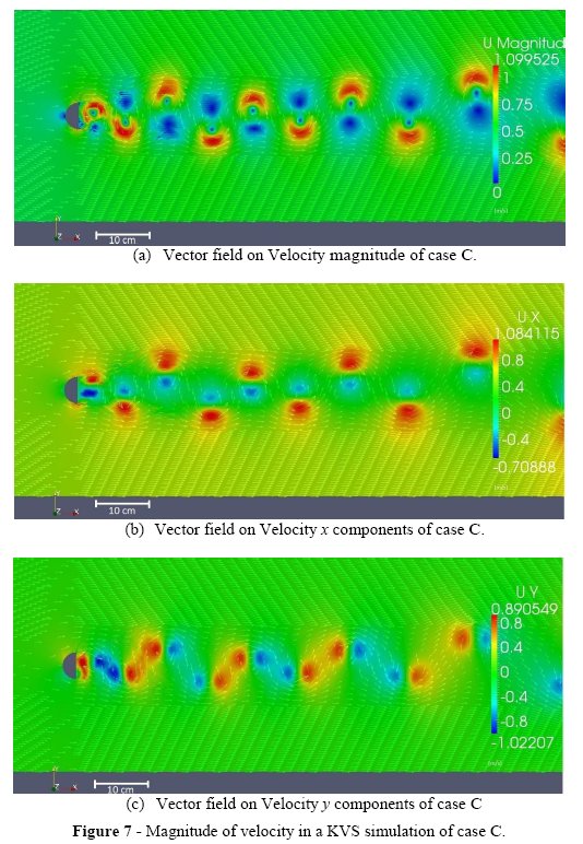
It can be observed that the asymmetry doesn’t correspond directly to the laminar  flow velocity  but  the  medium  point  between Uxmax and  Uxmin from Table  2 falls in a  value  around  0.35 for vortices  from 4 to  6 that   corresponds  to the core velocity measured  in  simulations. So, instead of extracting the laminar flow from these simulations, we extracted this Uvx flow and obtained a symmetrical behaviour of the regions inside the vortices. In figure 8 we show the flow without Uvx.

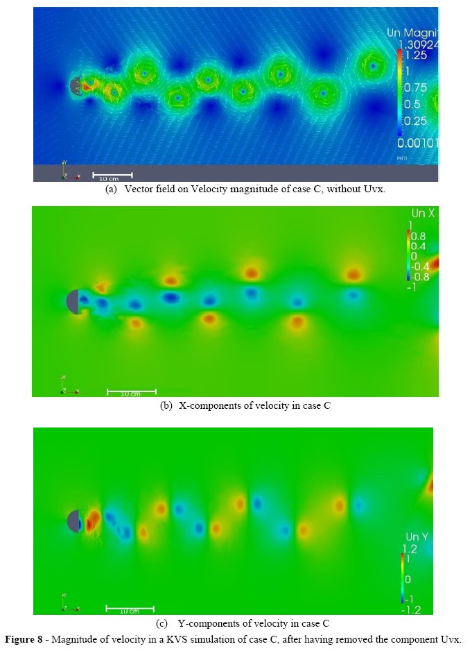
Figure 7(a) shows the  graphical  representation of a 2 dimensional simulation  of case C with  the  vectors  showing the  direction  of the  flow.  7(b) shows the same simulation step but only x components of the flow and 7(c) shows the same simulation step but only y components of the flow.

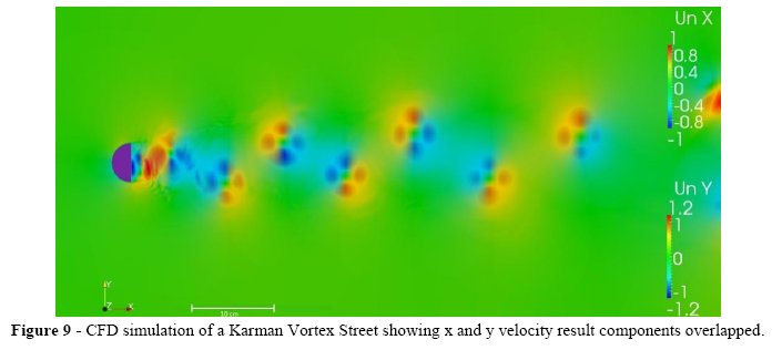
•  OVERLAPPED REPRESENTATION: If we take figures 8(b) and 8(c) and over-lap them making, for example, the 0 velocity value area of the y component become transparent, we obtain  the  image  shown in figure 9,  where  the regions X+ , X−,  Y+  and Y−  become clear.

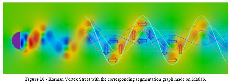
Using a Matlab representation as the one of Figure 6 and overlapping it to a segmented representation of a CFD simulation as the one of Figure 9, we obtain Figure 10. This Figure has been created only to illustrate the region where the values and equations presented in this work are valid and shows the coincident regions where the resultant velocity components in x and y are extracted for the model.

4.1 VALIDATION

The process of validation of the model is focused on the behaviour along time in steady state in specific points inside the Karman Vortex Street. What we try to show here is a comparison of the global behaviour of the velocity components of CFD simulations and our model along time.

To better compare the behaviour of the model with the real flow, meaning the difference between a full model and our simplified approach, we performed some statistics comparisons along time. Domain data was extracted from points located on a line transversal to the flow in the region of action of the model, as seen in Figure 11, for both, CFD and the Matlab model.

As the values of velocity components are calculated based on extracted data from CFD simulations, this parameter is not going to be discussed. Instead, the cyclic behaviour and change of direction of the flow is going to be analysed and compared to show the validity of this model.

The method used here was as follows:

•  SAMPLING POINT'S SELECTION: In each simulation case three points were defined along x axis:

P12 Corresponding to the average x coordinates of the centre of the second vortex detected in the selected region.

P22 Corresponding to the average x coordinates of the centre of the third vortex detected in the selected region. Or Pi0 + λ

Then, 4 equally distributed points were disposed along the y axis of these points. The distance between them corresponds to 1 d obtained from Table 2. Table 4 shows the coordinates of these points and Figure 11 show the location of them in CFD simulations and Matlab simulations.

•  DATA EXTRACTED: Values of velocity in x and y were obtained for at least 4 vortex cycles from CFD and Matlab simulations at the points selected (Table 4).

The representation of the magnitude of the velocity components alongtime on the points selected and shown in Figure 11 shows an evident analogous pattern. As an example we show in Figure 12 the CFD and the Matlab.

]]> The representation of the magnitude of the velocity components along time on the points selected and shown in Figure 11 shows an evident analogous pattern. As an example we show in Figure 12 the CFD and the Matlab results of the velocity magnitude at point P01 of case C where the similarity in the patterned behaviour manifests itself.

We can observe that the behaviour of the velocity components in both cases is highly correlated as can be seen in Figure 13.The highest correlation value corresponds to the main vortex shedding frequency as it could be expected.

4.2    EXAMPLE ON A FISH-LIKE ROBOT SIMULATION

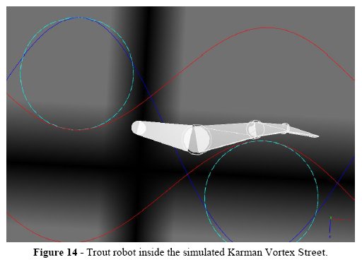
In order to show the application  of this set of values and equations  that  we presented  in this article,  we built a simulation of a trout-like  robot that  will be inserted  inside a Karman  street.  The simulations of the system “robot - Karman Street” have been performed in Webots [22].

•  THE ROBOT: We simulated a 0.1 m long trout robot with three articulations, as seen in Figure 14. The robot is controlled  by oscillators that  tune themselves to the vortex shedding frequency of the Karman  Street  allowing the  robot  to hold station  inside the  desired region of The  Karman  Street.

•  PHYSICS PLUGIN: The Karman Street has been simulated with a plug-in that calculates the forces from the water on the body of the robot. For this case the static drag approximation was used (no added mass). The main parameters used are shown in Table 5.

The results obtained show the forces on the bodies of the robot while it tries to hold station between vortices 4 to 6. The lateral and longitudinal forces are illustrated in Figures 15 and 16, respectively.

The plug-in calculates the velocity of the body relative to the water, converting it into a drag force against the direction of motion of each body.

5.     CONCLUSIONS

Although  this  method  doesn’t  take  on  account the  effect of the  rigid body on the flow, it gives the information  that  the robot controller needs to adapt  to the flow, allowing the training  phase and to obtain  a quite realistic simulation  of the robot behaviour inside a Karman  Vortex Street.

The continuous aspect and sinusoidal representation of the Karman Street was also a desired aspect of it. This was meant to search in a future the equilibrium of the oscillatory system KVS - Fish as it seems to behave as an oscillatory system in normal mode when the fish tunes its body to perform the Karman gait [23].

We found our method in a successful match with CFD simulations and used the CFD main values to fill the sections with the flow velocity components.  The validation was performed with CFD simulations for specific cases of which we had experimental data. The examples with the trout robot showed a reasonable behaviour in agreement with experimental real fish data [20].

From the robotics evolutionary control perspective it would be interesting to extend the model to further regions.  This could be done by including the damping effect that is observed in further regions than the one studied here, keeping the degree of simplicity of the model.  A wider statistical approach with more CFD cases to fit the waves to data could help making this a more standard method and of a wider application area.

6.     REFERENCES

[1] M. J. Lighthill. Large-amplitude elongated-body theory of fish locomotion.Proceedings of the Royal Society of London. Series B, Biological Sciences, 179 - 1055:125 – 138, 1971.

[2] S. Galls and O. Rediniotis. Neural network navigation of a biomimetic underwater vehicle. In Aerospace Sciences Meeting and Exhibit, 2001.

[3] S. F. Galls and O. K. Rediniotis. Development of a computational hydrodynamic model fora biomimetic underwaterautonomous vehicle. AIAA JOURNAL, 45-5, 2007.

[5] M. Porez. Modele dynamique analytique de la nage tridimensionnelle anguilliforme pour la robotique. PhD thesis, Ecole des Mines de Nantes,2007.        [ Links ]

[6] O. Ekeberg. A combined neuronal and mechanical model of fish swimming. Biological Cybernetics, 69:363–374, 1993.         [ Links ]

[7] A. Ijspeert. A connectionist central patterngenerator forthe aquatic and terrestrial gaits of a simulated salamander.   Biological cybernetics, 84:331–348, 2001.         [ Links ]

[8] D. Adkins and Y. Y. Yan. CFDsimulation of fish-like body moving in viscous liquid.Journal of Bionic Engineering, 3:147–153, 2006.

[9] N. Vandenberghe, J. Zhang, and S. Childress. Symmetry breaking leads to forward flapping flight. J. Fluid Mech., 506:147–155, 2004.

[10] J.  Eldredge and D. Pisani.Passive locomotion of a simple articulated fish-like system in the wake of an obstacle. J. Fluid Mech., 607:279–288, 2008.

[11] E. Tytell, C. Hsu, T. Williams, A. Cohen, and L. Fauci. Interactions between internal forces, body stiffness, and fluid environment in a neuromechanical model of lamprey swimming.   PNAS, 107:19832–19837, 2010.

[12] G. K. Taylor, R. L. Nudds, and A. L. R. Thomas.  Flying and swimming animals cruise at a Strouhal number tuned forhigh power efficiency. Nature, 425:707–711, 2003.

[13] M. Triantafyllou and G. Triantafyllou. An efficient swimming machine. Scientific American, March, 1995.

[15] Th. V. Karman. Uber den mechanismusdes widerstandes, den ein bewegter korper in einer flussigkeit erfahrt. Nachrichten von der Gesellschaft der Wissenschaften zu Gottingen, Mathematisch- Physikalische Kl., pages 509–517, 1911.

[16] Th. V. Karman. Uber den mechanismusdes widerstandes, den ein bewegter korper in einer flussigkeit erfahrt.  Nachrichten von der Gesellschaft der Wissenschaften zu Gottingen, Mathematisch- Physikalische Kl., pages 547–556, 1912

[17] James Carl Schatzman.  A model for the Von Karman vortex street.  PhD thesis, Applied mathematics - California Institute of technology, 1981.

[18] H. Helmholtz. On the integrals of the hydrodynamical equations which express vortex motion. The London, Edinburgh and Dublin Philosophical magazine and journal ofscience. 33:485–511, 1867.        [ Links ]

[19] O.Pust and C. Lund. Laser Techniques Applied to Fluid Mechanics, chapter Turbulent shear flows - The Karman VortexStreet - LDV and PIV Measurements Compared with CFD, pages 129–142. Springer, Berlin, 2000.

[20] J. Liao, D. Beal, G. Lauder, and M. Triantafyllou.The Karman gait: novel body kinematics ofrainbow trout swimming in a vortex street. The journal of experimental biology, 206:1059–1073, 2003.

[21] J. Liao, D. Beal, G. Lauder, and M. Triantafyllou. Fish exploiting vortices decrease muscle activity. Science, 302:1566–1569, 2003.

[22] Webots. Commercial Mobile Robot Simulation Software.        [ Links ]

[23] C.Tapia-Siles and R.Chellali. Simulation of an under-actuated fish-like robot controlled by an adaptive frequency oscillator inside a Karman Vortex Street. IFAC Proceedings Volumes: (IFAC-PapersOnline). Vol. 31. ed. 2012. p. 19-24.