<?xml version="1.0" encoding="ISO-8859-1"?><article xmlns:mml="http://www.w3.org/1998/Math/MathML" xmlns:xlink="http://www.w3.org/1999/xlink" xmlns:xsi="http://www.w3.org/2001/XMLSchema-instance">
<front>
<journal-meta>
<journal-id>2074-4706</journal-id>
<journal-title><![CDATA[Revista Latinoamericana de Desarrollo Económico]]></journal-title>
<abbrev-journal-title><![CDATA[rlde]]></abbrev-journal-title>
<issn>2074-4706</issn>
<publisher>
<publisher-name><![CDATA[Universidad Católica Boliviana "San Pablo"]]></publisher-name>
</publisher>
</journal-meta>
<article-meta>
<article-id>S2074-47062014000200003</article-id>
<title-group>
<article-title xml:lang="en"><![CDATA[Social Impacts of Climate Change in Bolivia: A municipal level analysis of the effects of recent climate change on life expectancy, consumption, poverty and inequality]]></article-title>
<article-title xml:lang="es"><![CDATA[Impactos sociales del cambio climático en Bolivia: un análisis a nivel municipal de los efectos del cambio climático reciente sobre esperanza de vida, consumo, pobreza y desigualdad]]></article-title>
</title-group>
<contrib-group>
<contrib contrib-type="author">
<name>
<surname><![CDATA[Andersen]]></surname>
<given-names><![CDATA[Lykke E.]]></given-names>
</name>
<xref ref-type="aff" rid="A01"/>
</contrib>
<contrib contrib-type="author">
<name>
<surname><![CDATA[Verner]]></surname>
<given-names><![CDATA[Dorte]]></given-names>
</name>
<xref ref-type="aff" rid="A02"/>
</contrib>
</contrib-group>
<aff id="A01">
<institution><![CDATA[,Institute for Advanced Development Studies (INESAD)  ]]></institution>
<addr-line><![CDATA[La Paz ]]></addr-line>
<country>Bolivia</country>
</aff>
<aff id="A02">
<institution><![CDATA[,Office of Evaluation and Oversight, Inter-American Development Bank  ]]></institution>
<addr-line><![CDATA[Washington D.C.]]></addr-line>
</aff>
<pub-date pub-type="pub">
<day>00</day>
<month>11</month>
<year>2014</year>
</pub-date>
<pub-date pub-type="epub">
<day>00</day>
<month>11</month>
<year>2014</year>
</pub-date>
<numero>22</numero>
<fpage>49</fpage>
<lpage>83</lpage>
<copyright-statement/>
<copyright-year/>
<self-uri xlink:href="http://www.scielo.org.bo/scielo.php?script=sci_arttext&amp;pid=S2074-47062014000200003&amp;lng=en&amp;nrm=iso"></self-uri><self-uri xlink:href="http://www.scielo.org.bo/scielo.php?script=sci_abstract&amp;pid=S2074-47062014000200003&amp;lng=en&amp;nrm=iso"></self-uri><self-uri xlink:href="http://www.scielo.org.bo/scielo.php?script=sci_pdf&amp;pid=S2074-47062014000200003&amp;lng=en&amp;nrm=iso"></self-uri><abstract abstract-type="short" xml:lang="en"><p><![CDATA[This paper analyzes the direct evidence of climate change in Bolivia during the last 60 years, and estimates how these changes have affected life expectancy and consumption levels for each of the 311 municipalities in Bolivia. Contrary to the predictions of most General Circulation models, the evidence shows a consistent cooling trend of about 0.2ºC per decade over all highland areas, slight and scattered evidence of warming in the lowlands, and no systematic changes in precipitation. The estimations indicate that the 1ºC cooling experienced in the already cold highlands over the last five decades likely has reduced consumption possibilities by about 2-3% in these areas. Since the much richer population in the lowlands have benefitted slightly from recent climate change, our simulations suggest that recent climate change has contributed to an increase in inequality and poverty in Bolivia. Poor and indigenous peoples in the highlands are among the most severely affected populations. No statistically significant effect on life expectancy was found.]]></p></abstract>
<abstract abstract-type="short" xml:lang="es"><p><![CDATA[Este estudio analiza la evidencia directa del cambio climático en Bolivia durante los últimos 60 años y realiza una estimación de los efectos de estos cambios sobre la esperanza de vida y el nivel de consumo en cada uno de los 311 municipios de Bolivia. En contradicción con la mayoría de los modelos de circulación global, la evidencia directa muestra una tendencia consistente de enfriamiento de aproximadamente 0.2ºC por década en el Altiplano, evidencia esporádica de calentamiento en las tierras bajas, y ninguna tendencia sistemática en las precipitaciones. Las estimaciones indican que el enfriamiento observado de 1ºC en las áreas ya frías del Altiplano durante las últimas cinco décadas probablemente ha reducido el nivel de consumo en 2-3 por ciento en estas áreas. Dado que la población más rica de las tierras bajas se ha beneficiado levemente del cambio climático reciente, nuestras simulaciones sugieren que el cambio climático reciente ha contribuido a un aumento en la pobreza y la desigualdad en Bolivia. Los habitantes pobres e indígenas del Altiplano son los que más han sido afectados. No se ha encontrado un efecto significativo sobre la esperanza de vida.]]></p></abstract>
<kwd-group>
<kwd lng="en"><![CDATA[Climate change]]></kwd>
<kwd lng="en"><![CDATA[social impacts]]></kwd>
<kwd lng="en"><![CDATA[Bolivia]]></kwd>
<kwd lng="es"><![CDATA[Cambio climático]]></kwd>
<kwd lng="es"><![CDATA[impactos sociales]]></kwd>
<kwd lng="es"><![CDATA[Bolivia]]></kwd>
</kwd-group>
</article-meta>
</front><body><![CDATA[ <p align="center">&nbsp;</p>     <p align="center">&nbsp;</p>     <p align="center"><b><font size="4" face="Verdana, Arial, Helvetica, sans-serif">Social  Impacts of Climate    Change in  Bolivia: A municipal    level  analysis of the effects    of recent  climate change on    life  expectancy, consumption,    poverty and  inequality</font></b></p>     <p align="center">&nbsp;</p>     <p align="center"><b><font size="3" face="Verdana, Arial, Helvetica, sans-serif">Impactos sociales del cambio clim&aacute;tico   en Bolivia: un an&aacute;lisis a nivel municipal   de los efectos del cambio clim&aacute;tico    reciente sobre esperanza de vida,    consumo, pobreza y desigualdad</font></b></p>     <p align="center">&nbsp;</p>     <p align="center">&nbsp;</p>     <p align="center"><font size="2" face="Verdana, Arial, Helvetica, sans-serif">    <br>     <i><b>Lykke E. Andersen*</b></i><b>, <i>Dorte  Verner**</i></b></font></p>     <p align="justify">&nbsp;</p>     ]]></body>
<body><![CDATA[<p align="justify">&nbsp;</p> <hr noshade>     <p align="justify"><font size="2" face="Verdana, Arial, Helvetica, sans-serif"><b>Abstract</b></font></p>     <p align="justify"><font size="2" face="Verdana, Arial, Helvetica, sans-serif">This paper analyzes the direct evidence of climate  change in Bolivia during the last 60    years, and estimates how these changes have affected  life expectancy and consumption    levels for each of the 311 municipalities in Bolivia.  Contrary to the predictions of most    General Circulation models, the evidence shows a  consistent cooling trend of about 0.2&ordm;C    per decade over all highland areas, slight and  scattered evidence of warming in the lowlands, and no systematic changes in precipitation. The estimations  indicate that the 1&ordm;C cooling    experienced in the already cold highlands over the  last five decades likely has reduced    consumption possibilities by about 2-3% in these  areas. Since the much richer population in    the lowlands have benefitted slightly from recent  climate change, our simulations suggest that   recent climate change has contributed to an increase  in inequality and poverty in Bolivia. Poor   and indigenous peoples in the highlands are among the  most severely affected populations.    <br>   No statistically significant effect on life expectancy  was found.</font></p>     <p align="justify"><font size="2" face="Verdana, Arial, Helvetica, sans-serif"><b> Keywords:</b> Climate change, social impacts, Bolivia.</font></p>     <p align="justify"><font size="2" face="Verdana, Arial, Helvetica, sans-serif"><b>Classification  JEL:</b> Q51, Q54, O15, O19, O54.</font></p> <hr noshade>     <p align="justify"><font size="2" face="Verdana, Arial, Helvetica, sans-serif"><b>  Resumen</b></font></p>     <p align="justify"><font size="2" face="Verdana, Arial, Helvetica, sans-serif">  Este  estudio analiza la evidencia directa del cambio clim&aacute;tico en Bolivia durante  los  &uacute;ltimos  60 a&ntilde;os y realiza una estimaci&oacute;n de los efectos de estos cambios sobre la  esperanza   de  vida y el nivel de consumo en cada uno de los 311 municipios de Bolivia. En  contradicci&oacute;n   con  la mayor&iacute;a de los modelos de circulaci&oacute;n global, la evidencia directa muestra  una    tendencia  consistente de enfriamiento de aproximadamente 0.2&ordm;C por d&eacute;cada en el  Altiplano,   evidencia  espor&aacute;dica de calentamiento en las tierras bajas, y ninguna tendencia  sistem&aacute;tica   en  las precipitaciones. Las estimaciones indican que el enfriamiento observado de  1&ordm;C en las  &aacute;reas  ya fr&iacute;as del Altiplano durante las &uacute;ltimas cinco d&eacute;cadas probablemente ha  reducido el   nivel  de consumo en 2-3 por ciento en estas &aacute;reas. Dado que la poblaci&oacute;n m&aacute;s rica de  las   tierras  bajas se ha beneficiado levemente del cambio clim&aacute;tico reciente, nuestras  simulaciones   sugieren  que el cambio clim&aacute;tico reciente ha contribuido a un aumento en la pobreza y la   desigualdad  en Bolivia. Los habitantes pobres e ind&iacute;genas del Altiplano son los que m&aacute;s han sido  afectados. No se ha encontrado un efecto significativo sobre la esperanza de  vida.</font></p>     <p align="justify"><font size="2" face="Verdana, Arial, Helvetica, sans-serif"><b> Palabras  clave:</b> Cambio clim&aacute;tico, impactos sociales,  Bolivia.</font></p>     <p align="justify"><font size="2" face="Verdana, Arial, Helvetica, sans-serif"><b>Clasificaci&oacute;n  JEL:</b> Q51, Q54, O15, O19, O54.</font></p> <hr noshade>     ]]></body>
<body><![CDATA[<p align="justify">&nbsp;</p>     <p align="justify">&nbsp;</p>     <p align="justify"><font size="3" face="Verdana, Arial, Helvetica, sans-serif">  <b>1. Introduction<sup>1</sup></b></font></p>     <p align="justify"><font size="2" face="Verdana, Arial, Helvetica, sans-serif">  Although Bolivia is located entirely within the  tropics, the large altitude variations within    the country imply that it has almost every conceivable  type of climate ranging from Andean   glaciers, via salt deserts, to steaming rainforest.  This variation makes Bolivia ideally suited for   an empirical analysis of the social impacts of climate  change because the limited variation in   the time dimension can be complemented by ample  variation in the spatial dimension.</font></p>     <p align="justify"><font size="2" face="Verdana, Arial, Helvetica, sans-serif">A simple way to gauge how climate affects human  development is to compare human   development across regions with different climates.  This has, for example, been done by   Horowitz (2006), which uses a cross-section of 156  countries to estimate the relationship   between temperature and income level. The overall  relationship found is very strongly   negative, with a 2&deg;F increase in global temperatures  implying a 13 % drop in income. This   is very dramatic, but the relationship is thought to  be mostly historical and thus not very   relevant for the prediction of the contemporary  effects of climate change in the recent past   or near future. In order to control for historical  factors, the paper includes colonial mortality   rates as an explanatory variable, and finds a much  more limited, but still highly significant,   contemporaneous effect of temperature on incomes. The  contemporaneous relationship   estimated implies that a 2&deg;F increase in global  temperatures would cause approximately a 3.5%   drop in World GDP.</font></p>     <p align="justify"><font size="2" face="Verdana, Arial, Helvetica, sans-serif">  In order to further control for historical  differences, Horowitz (2006) uses more   homogeneous sub-samples, such as one with only OECD  countries or only countries from   the Former Soviet Union, and the negative relationship  still holds. However, as directions for   further research, he recommends empirical studies of  income and temperature variations   within large, heterogeneous countries, which would  provide much more thorough control for   historical differences. This is exactly what we do in  this paper.</font></p>     <p align="justify"><font size="2" face="Verdana, Arial, Helvetica, sans-serif">  Using data from the 311 municipalities in Bolivia, we  estimate contemporary relationships   between temperature and consumption levels (a proxy  for income), as well as between   temperature and life expectancy. These relationships  are then used to gauge the likely direction   and magnitude of effects of climate change in Bolivia.</font></p>     <p align="justify"><font size="2" face="Verdana, Arial, Helvetica, sans-serif">  The rest of the paper is organized as follows. Section  2 describes the data and the sources.    Section 3 estimates municipal level econometric models  of the relationships between climate   variables, life expectancy, and consumption levels.  Section 4 analyzes climate change in Bolivia   from 1948 to 2008. Section 5 uses the estimated models  from Section 3 to simulate the effect   of recent climate change (from Section 4) on  consumption levels, poverty and inequality.    <br>   Finally, Section 6 concludes.</font></p>     <p align="justify">&nbsp;</p>     ]]></body>
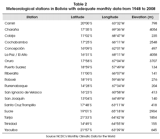
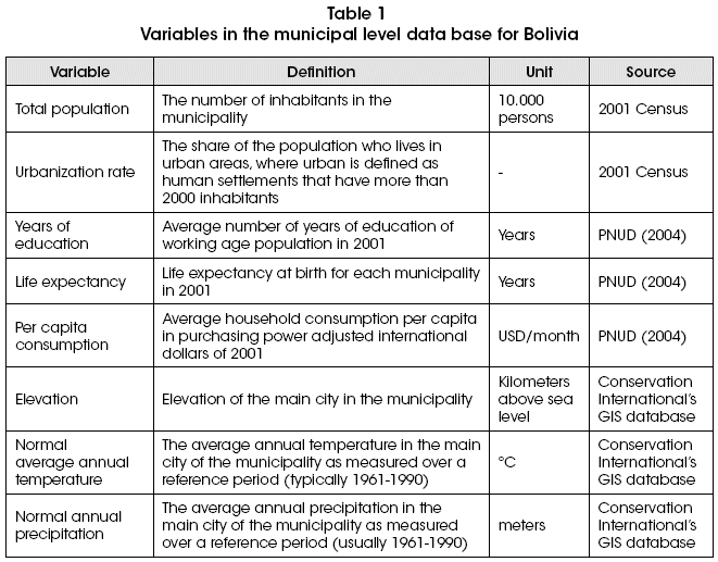
<body><![CDATA[<p align="justify"><font size="3" face="Verdana, Arial, Helvetica, sans-serif">  <b>2. The data</b></font></p>     <p align="justify"><font size="2" face="Verdana, Arial, Helvetica, sans-serif">  The data used for this paper consists of both  cross-section and time series data. The   municipal level cross-section data base used to  estimate the relationships between climate,   development and migration in Bolivia is constructed  using data from several different sources.    <br>   <a href="#t1">Table 1</a> lists the variables, their definitions and the  sources of the information.</font></p>     <p align="justify"><font size="2" face="Verdana, Arial, Helvetica, sans-serif"><a name="t1"></a></font></p>     <p align="center"><font size="2" face="Verdana, Arial, Helvetica, sans-serif"><img src="/img/revistas/rlde/n22/a03_table_01.gif" width="661" height="517">    <br>   </font></p>     <p align="justify"><font size="2" face="Verdana, Arial, Helvetica, sans-serif">In order to assess the climate change trends in the  different parts of Bolivia, we obtained    monthly temperature and precipitation data from 1948  to 2008 from the Monthly Climatic   Data for the World (MCDW), publication of the US  National Climatic Data Center<sup>2</sup>. The   original data is organized in 61 printed volumes with  12 issues in each (one for each month   of the year), totaling 721 months. All data has been  quality-checked and was published by the   NCDC about 3 months after the raw data has been  collected. From each of these monthly   issues, we extracted average monthly temperature and  total monthly for each of 31 Bolivian   stations, in order to create time series for each  station.</font></p>     <p align="justify"><font size="2" face="Verdana, Arial, Helvetica, sans-serif">  The &ldquo;normal&rdquo; temperature for each station-month is  calculated as the average temperature   observed for the reference period 1960-90. Some  stations have so few and scattered   observations that it is not feasible to calculate  reliable &ldquo;normal&rdquo; temperatures, and these   stations have therefore been discarded. Only the  stations that have at least eight observations   for each calendar month during the reference period  were included in the analysis in this   paper. An additional requirement for inclusion of a  data station in the present analysis is that it   has at least 300 out of the 721 possible monthly  observations. The 18 stations that satisfy both   of these requirements are listed in <a href="#t2">Table 2</a>.</font></p>     <p align="justify"><font size="2" face="Verdana, Arial, Helvetica, sans-serif"><a name="t2"></a></font></p>     <p align="center"><img src="/img/revistas/rlde/n22/a03_table_02.gif" width="665" height="580"></p>     ]]></body>
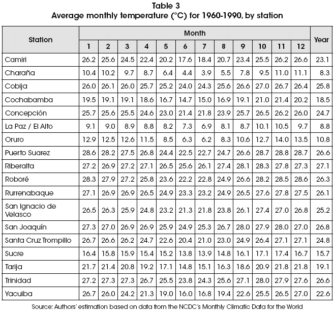
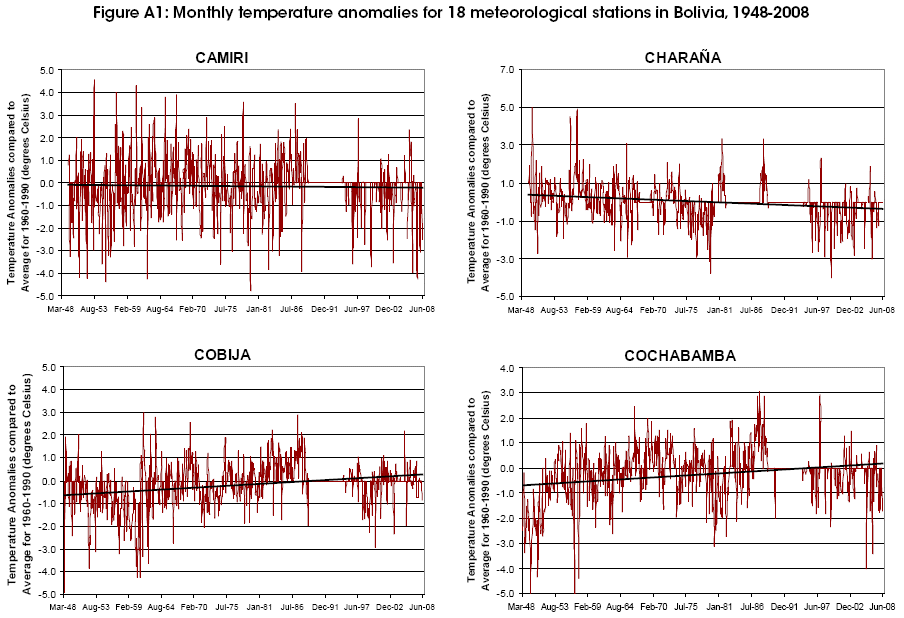
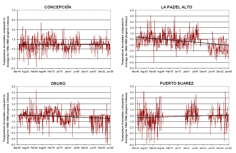
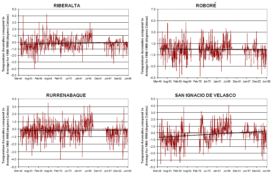
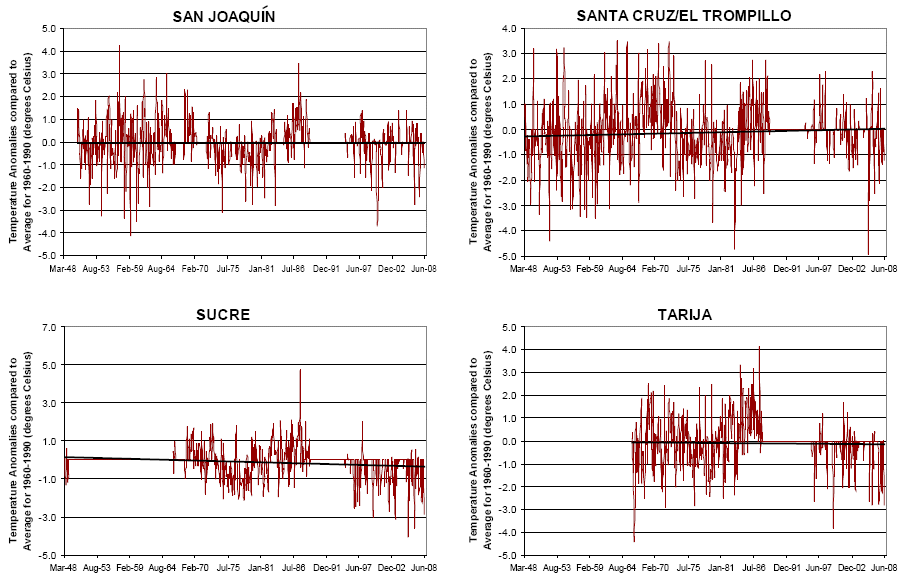
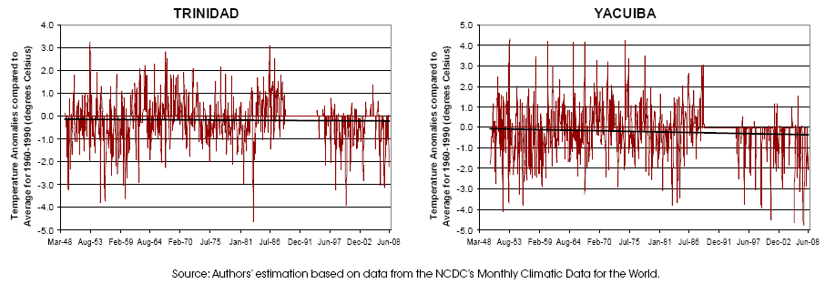
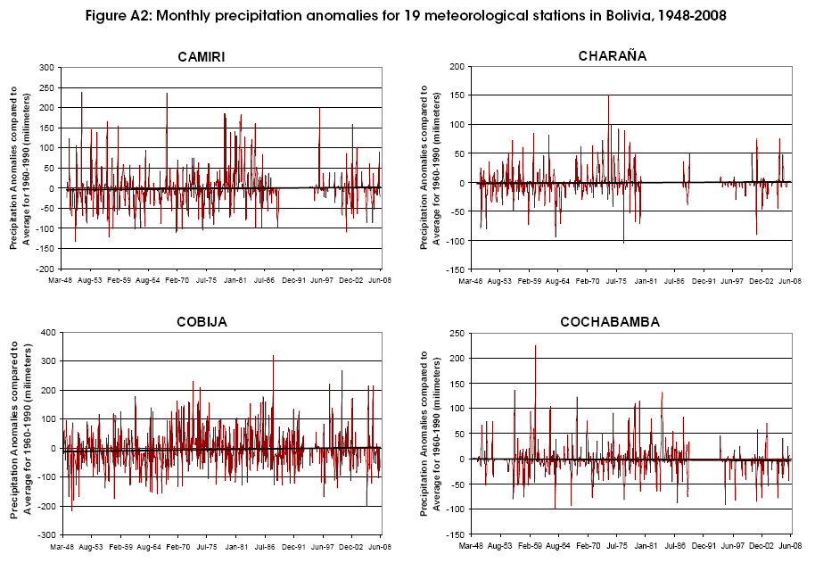
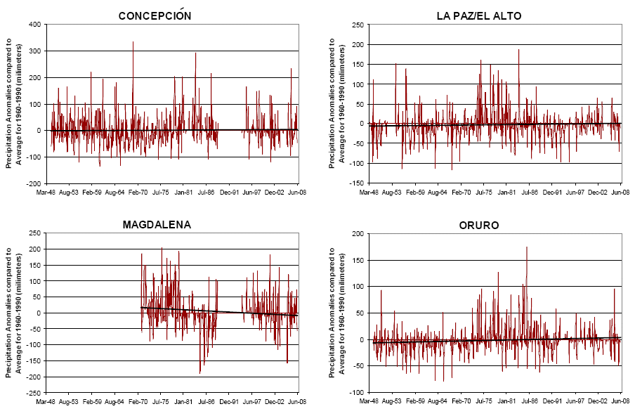
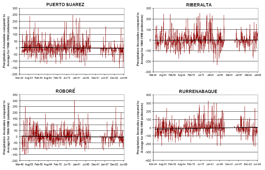
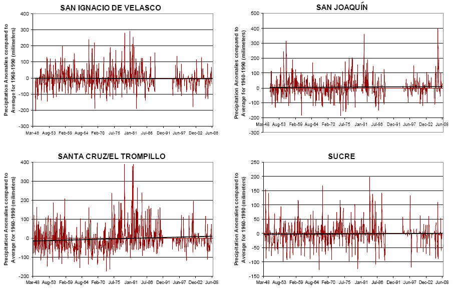
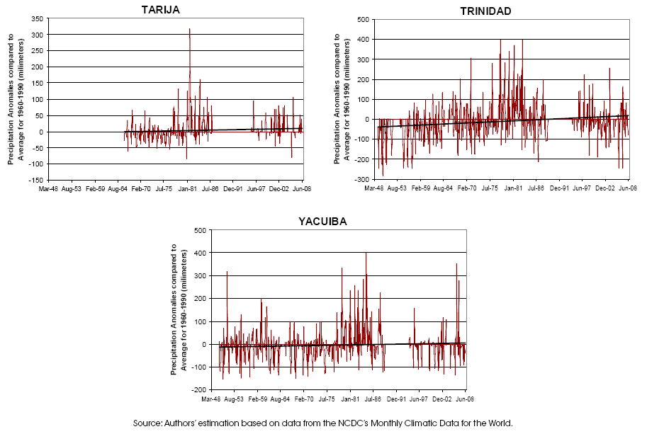
<body><![CDATA[<p align="justify"><font size="2" face="Verdana, Arial, Helvetica, sans-serif">    <br>     <a href="#t3">Table 3</a> shows the average &ldquo;normal&rdquo; temperatures for  each month for each of these stations.    <br>   It is seen that the climate differs dramatically from  region to region, with Chara&ntilde;a in the far   west being cold throughout the year due to the high  elevation, while most low-land regions are   hot throughout the year due to the location close to  the Equator.</font></p>     <p align="justify"><a name="t3"></a></p>     <p align="center"><img src="/img/revistas/rlde/n22/a03_table_03.gif" width="659" height="615"></p>     <p align="justify"><font size="2" face="Verdana, Arial, Helvetica, sans-serif">  The difference in temperature between the warmest and  the coldest month also varies. In   Cobija and Riberalta, for example, the difference  between the warmest and the coldest month   is less than 3&ordm;C. Yacuiba is the southernmost station  in Bolivia and therefore the station that   shows the most marked temperature variations over the  year, but the difference between the   warmest and the coldest month is still only 11&ordm;C.</font></p>     <p align="justify"><font size="2" face="Verdana, Arial, Helvetica, sans-serif"> Using the &ldquo;normal&rdquo; values for each station and each  month, we calculate monthly anomalies   for each station for the whole period (actual  temperature minus normal temperature for that   month). Anomalies are easier to analyze than the raw  temperature and precipitation data, since   the seasonal variation is eliminated through the  subtraction of normal monthly temperatures.</font>    <br>   <font size="2" face="Verdana, Arial, Helvetica, sans-serif"><a href="#fa1">Figure A1</a> in the Annex plots the temperature anomalies  for each station.</font></p>     <p align="justify"><font size="2" face="Verdana, Arial, Helvetica, sans-serif">  The precipitation data applied in the analyses have  been subjected to the same procedure,    and all precipitation anomalies are plotted in <a href="#fa2">Figure  A2</a> of the Annex.</font></p>     <p align="justify">&nbsp;</p>     ]]></body>
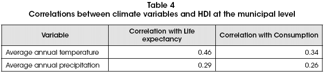
<body><![CDATA[<p align="justify">  <font size="3" face="Verdana, Arial, Helvetica, sans-serif"><b>3. Modeling climate and human  development</b></font></p>     <p align="justify"><font size="2" face="Verdana, Arial, Helvetica, sans-serif">  Bolivia is a very heterogeneous country both with  respect to climate and with respect to   development. Some regions have extremely harsh  climates with sub-zero temperatures most   of the year and very little rain. Other regions are  hot and constantly humid. Some people live   in remote areas without road access in simple one-room  dwellings without electricity, piped   water, bathroom, or any other basic conveniences.  Other people live in mansions with home   cinema, swimming pool, fitness room, and servants.</font></p>     <p align="justify"><font size="2" face="Verdana, Arial, Helvetica, sans-serif">  This variation makes Bolivia ideally suited for  estimating the impact of climate on   development, as the limited variation in time can be  complemented by ample variation in   space, while still holding the most important  confounding variables constant.</font></p>     <p align="justify"><font size="2" face="Verdana, Arial, Helvetica, sans-serif">  As proxies for human development, we will use the  following two variables: (i) life   expectancy at birth, and (ii) consumption <i>per capita</i>.</font></p>     <p align="justify"><font size="2" face="Verdana, Arial, Helvetica, sans-serif">  Across the 311 municipalities in Bolivia, life  expectancy at birth varies between 40 and   70 years, while annual consumption <i>per capita </i>varies between US$ 245 and US$ 2,565   (purchasing power adjusted international dollars of  the year 2001).</font></p>     <p align="justify"><font size="2" face="Verdana, Arial, Helvetica, sans-serif">  The variables of principal interest are the climate  variables: average temperature and   average precipitation. Simple correlations between  these and the two human development   variables are presented in <a href="#t4">Table 4</a>. According to these  simple correlations, warm and wet is   good, while cold and dry is bad for human development.</font></p>     <p align="justify"><a name="t4"></a></p>     <p align="center"><img src="/img/revistas/rlde/n22/a03_table_04.gif" width="656" height="148"></p>     <p align="justify"><font size="2" face="Verdana, Arial, Helvetica, sans-serif">In order to control for other differences between  municipalities, we include the climate   variables in a regression framework together with two  important control variables: Education   levels and urbanization rates, which are both unlikely  to be affected by climate changes in the   short run, but are clearly related to life expectancy  and consumption levels. It is also important   to allow for non-linear effects, as both too high and  too low temperatures may be unfavorable   for human development, just as both too much and too  little rain may cause problems (<i>e.g</i>.   Mendelsohn, Nordhaus &amp; Shaw, 1994; Quiggin &amp;  Horowitz, 1999; Masters &amp; McMillan, 2001; Tol, 2005).</font></p>     <p align="justify"><font size="2" face="Verdana, Arial, Helvetica, sans-serif">  Thus, the regressions in this section will take the  following form:</font></p>     ]]></body>
<body><![CDATA[<p align="center"><img src="/img/revistas/rlde/n22/a03_ecuacion_01.gif" width="658" height="39"></p>     <p align="justify"><font size="2" face="Verdana, Arial, Helvetica, sans-serif">where <i>c<sub>i</sub> </i>is a measure  of the consumption level in municipality <i>i</i>, <i>temp<sub>i</sub> </i>and <i>rain<sub>i</sub> </i>are normal   average annual temperature and normal accumulated  annual precipitation in municipality <i>i</i>,   <i>edu<sub>i</sub> </i>is a measure of the education  level (average years of schooling of the population aged   15 and older), <i>urb<sub>i</sub> </i>is the urbanization rate of the  municipality, and <i>&epsilon;<sub>i</sub> </i>is the error term for   municipality <i>i</i>.   </font></p>     <p align="justify"><font size="2" face="Verdana, Arial, Helvetica, sans-serif">The life expectancy regression will take the same form  as the consumption regression,   except that we will not apply the natural logarithm to  the dependent variable. Both regressions are weighted OLS regressions, where the weights  consist of the population size in each   municipality. The regression results for both  consumption and life expectancy are reported    in <a href="#t5">Table 5</a>.</font></p>     <p align="justify"><font size="2" face="Verdana, Arial, Helvetica, sans-serif"><a name="t5"></a></font></p>     <p align="center"><img src="/img/revistas/rlde/n22/a03_table_05.gif" width="564" height="556"></p>     <p align="justify"><font size="2" face="Verdana, Arial, Helvetica, sans-serif">The results at the bottom of the table show that just  these four explanatory variables   (temperature, precipitation, education and  urbanization rates) explain 92% of the variation in   consumption levels between the municipalities in  Bolivia. This is an extremely good fit, which   suggests that we have included the most important  explanatory variables, and that including   additional variables would make little difference. The  same four variables only explain about   74 5% of the variation in life expectancy, which is  less impressive, but still very good for a crosssection model.</font></p>     <p align="justify"><font size="2" face="Verdana, Arial, Helvetica, sans-serif">  Education is by far the most important variable,  explaining about 88% of the variation    in consumption levels and about 54% of the variation in  life expectancy. Urbanization rates are also significant in both regressions, in a  non-linear manner that suggests that the optimal   urbanization rate is around 70% for consumption and  about 50% for life expectancy.</font></p>     <p align="justify"><font size="2" face="Verdana, Arial, Helvetica, sans-serif">  The temperature variables are highly significant in  explaining consumption, but not life    expectancy. Precipitation is not significant in any of  the regressions. As it is difficult to assess   the non-linear effects of temperature directly by  looking at the estimated coefficients, we   have plotted the estimated relationship in <a href="#f1">Figure 1</a>.  The axes are scaled to represent the actual   range of temperatures and consumption levels in  different Bolivian municipalities, so that the   magnitude of climate impacts can be seen in the  appropriate perspective. A 95% confidence   interval on the temperature-consumption relationship  is also indicated in the graph.</font></p>     <p align="justify"><a name="f1"></a></p>     <p align="center"><img src="/img/revistas/rlde/n22/a03_figure_01.gif" width="421" height="418"></p>     ]]></body>
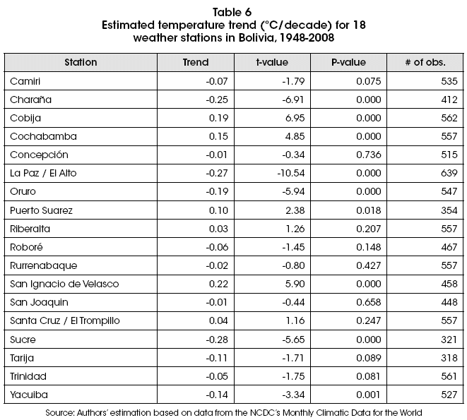
<body><![CDATA[<p align="justify"><font size="2" face="Verdana, Arial, Helvetica, sans-serif">    <br>   The estimated relationship indicates that Bolivians do  considerably better in hot areas   than in cold areas, even when controlling for other  factors such as education attainment   and urbanization levels. Inhabitants in the hottest  regions are able to consume almost twice   as much as inhabitants in the coldest regions. The  slope is decreasing with temperature,   suggesting that already hot areas would benefit only  little in terms of consumption from   additional increases in temperature, whereas presently  cold areas would benefit more.</font></p>     <p align="justify"><font size="2" face="Verdana, Arial, Helvetica, sans-serif">Having established that temperature has an important  effect on consumption possibilities   in Bolivia, we will now proceed to test whether there  have been any significant changes in temperatures in Bolivia during the last 6 decades.</font></p>     <p align="justify">&nbsp;</p>     <p align="justify"><font size="3" face="Verdana, Arial, Helvetica, sans-serif">  <b>4. Recent climate change in  Bolivia</b></font></p>     <p align="justify"><font size="2" face="Verdana, Arial, Helvetica, sans-serif">  In this section we will analyze climate data from the  18 meteorological stations of highest   quality in Bolivia from May 1948 to May 2008 to test  whether there are any significant trends,   and whether these trends differ between regions.</font></p>     <p align="justify"><font size="2" face="Verdana, Arial, Helvetica, sans-serif">  The actual measured temperatures are first converted  into temperature anomalies, by   subtracting the average &ldquo;normal&rdquo; temperature for each  station-month, as calculated for the   reference period 1960-90. All the temperature anomaly  series are plotted in <a href="#fa1">Figure A1</a> in the    Annex.</font></p>     <p align="justify"><font size="2" face="Verdana, Arial, Helvetica, sans-serif">  Once we have the series of temperature anomalies, it  is straightforward to test whether   there is a significant trend. This is done by  regressing the anomaly on a trend-variable which   has been scaled so that the coefficient can be  directly interpreted as temperature change per   decade in degrees Celsius. We use a confidence level  of 95% to decide whether the trend is   statistically significant, which means that the  P-value of the trend coefficient should be less   than 0.05 for the trend to be significant.</font></p>     <p align="justify"><font size="2" face="Verdana, Arial, Helvetica, sans-serif"><a href="#t6"> Table 6</a> shows the estimated trends in temperatures for  each of the 18 stations in Bolivia.</font>    <br>   <font size="2" face="Verdana, Arial, Helvetica, sans-serif">Of these, four stations show significant warming since  the middle of the previous century and nine show no significant change, and 5 show  significant cooling.</font></p>     ]]></body>
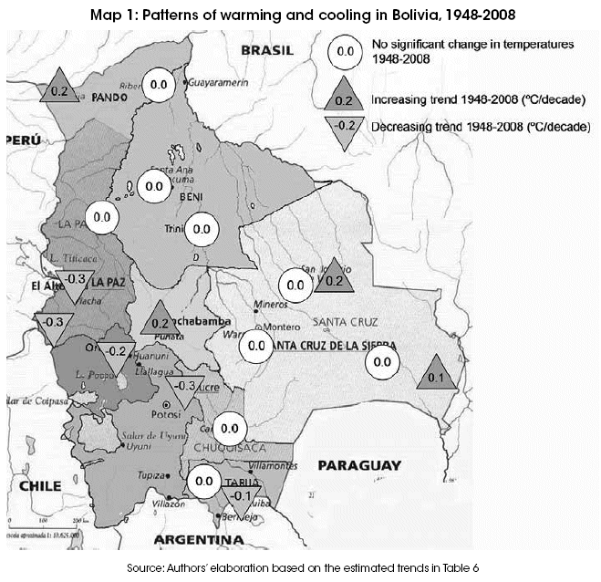
<body><![CDATA[<p align="justify"><a name="t6"></a></p>     <p align="center"><img src="/img/revistas/rlde/n22/a03_table_06.gif" width="661" height="595"></p>     <p align="justify"><font size="2" face="Verdana, Arial, Helvetica, sans-serif">None of the stations in Bolivia get even close to  having observations for all the 721   months in the 1948-2008 period, but some stations have  reported more consistently than   others. If we limit ourselves to the 15 stations that  have at least 400 observations, we find that   three show significant warming, four show significant  cooling, and eight show no significant   trend. A similar distribution is found if we limit  ourselves to the 11 stations that have at least 500 observations.</font></p>     <p align="justify"><font size="2" face="Verdana, Arial, Helvetica, sans-serif">The patterns of warming/cooling show a distinct  geographical distribution, with the   highland stations in the southwestern part of Bolivia  showing consistent cooling, and the   lowland areas to the north and east showing slight  warming (<a href="#m1">Map 1</a>). This is consistent with   NCDC data from neighboring countries, which show  cooling in many parts of Peru and   Chile but warming in Brazil (Andersen, Suxo &amp;  Verner, 2009; Andersen &amp; Verner 2009 and Andersen, Rom&aacute;n &amp; Verner, 2009).</font></p>     <p align="justify"><a name="m1"></a></p>     <p align="center"><img src="/img/revistas/rlde/n22/a03_map_01.gif" width="659" height="638"></p>     <p align="justify"><font size="2" face="Verdana, Arial, Helvetica, sans-serif">Since the data from any single station is subject to  idiosyncratic influences, it is necessary   to average over several stations in order to get  reliable results. In the case of Bolivia, the data   suggests that highland areas in general have  experienced cooling over the last 60 years, with an   average trend around -0.2&ordm;C/decade. For the purposes  of the simulations in the next section,   we will therefore assume a uniform cooling trend of  0.2&ordm;C/decade for all municipalities   located in the departments of Tarija, Chuquisaca,  Potos&iacute;, Oruro and the highland areas of La Paz (above 2000 meters above sea level).</font></p>     <p align="justify"><font size="2" face="Verdana, Arial, Helvetica, sans-serif">  For the lowland areas the evidence shows mostly no  significant trends, but interspersed   with a few positive trends. For the purposes of the  simulations in the next section, we will   assume a slight warming trend of 0.05&ordm;C/decade in all  lowland areas.</font></p>     <p align="justify"><font size="2" face="Verdana, Arial, Helvetica, sans-serif">  The general cooling of the highlands appears to be  inconsistent with the rapid melting   of several Bolivian glaciers, especially the  Chacaltaya and the Zongo glaciers close to El Alto   (Francou, Ramirez, Caceres &amp; Mendoza<i>, </i>2000, and Ramirez, Francou,  Ribstein, Descloitres,   Guerin, Mendoza, Gallaire, Pouyaud &amp; Jordan,  2001), but it is not. First of all, the glaciers   have been melting continuously since the Little Ice  Age (about 1550 to 1850), with only a   brief slowdown during the relatively cool period of  1950-1980, and it is normal for melting to   accelerate towards the end (just like a small ice cube  melts faster than a big ice cube).</font></p>     <p align="justify"><font size="2" face="Verdana, Arial, Helvetica, sans-serif">  In addition, glaciers depend on other factors than  temperature, notably precipitation, but   also cloud cover, relative humidity and the intensity  of solar irradiation (Ramirez, 2008). A   study of oxygen isotope series generated from ice  cores from two Bolivian glaciers suggests   that precipitation has decreased steadily since about  1974 (Hoffman, Ramirez, Taupin,   Francou, Ribstein, Delmas, D&uuml;rr, Gallaire, Sim&otilde;es,  Schotterer, Stievenard &amp; Werner, 2003)<sup>3</sup>.</font></p>     ]]></body>
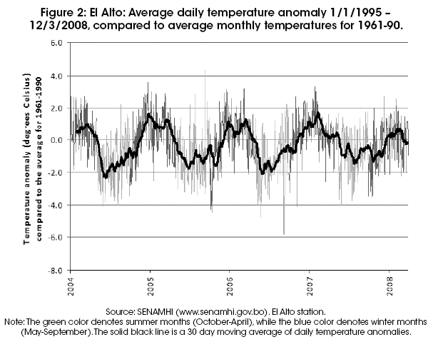
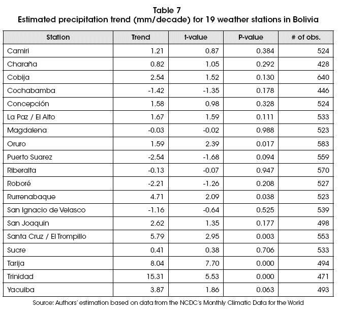
<body><![CDATA[<p align="justify"><font size="2" face="Verdana, Arial, Helvetica, sans-serif">  The reduction in precipitation is likely associated  with the general reduction in cloud   cover over the tropics since measurements began in the  early 1980s<sup>4</sup>, and less clouds means   more intense solar irradiation, which accelerates  glacial melt. Decreased cloud cover at this   altitude also works to amplify the diurnal temperature  range, increasing daytime temperatures   (which would cause increased melting), but reducing  night-time temperatures even more   (because of the missing cloud-blanket), which explains  the reduction in average temperatures.</font></p>     <p align="justify"><font size="2" face="Verdana, Arial, Helvetica, sans-serif"> Moreover, upon closer inspection of the temperature  data, it becomes clear that   temperatures have not fallen equally throughout the  year. At the El Alto station, for example,   summer temperatures have been increasing and winter  temperatures decreasing (<a href="#f2">Figure 2</a>).</font></p>     <p align="justify"><font size="2" face="Verdana, Arial, Helvetica, sans-serif"><a name="f2"></a></font></p>     <p align="center"><font size="2" face="Verdana, Arial, Helvetica, sans-serif"><img src="/img/revistas/rlde/n22/a03_figure_02.gif" width="607" height="479"></font></p>     <p align="justify"><font size="2" face="Verdana, Arial, Helvetica, sans-serif">  Since winter is the dry season in El Alto, the lower  winter temperatures will provide little   benefit for the glaciers, which cannot accumulate mass  without snowfall. Instead, these   glaciers are much more sensitive to changes in summer  temperatures and precipitation. This   explains why the ENSO (El Ni&ntilde;o-Southern Oscillation)  has such a strong effect on Bolivian   glaciers. During ENSO&rsquo;s warm and dry phase (El Ni&ntilde;o),  the mass balances are always negative,   implying shrinking glaciers. In the cooler and more  humid La Ni&ntilde;a phase, the glaciers return   to equilibrium and sometimes show a small increase.  The increase in the glacier regression   rate since the end of the 1970s appears to coincide  with the Pacific shift of 1976, the date after    which the El Ni&ntilde;o event became more frequent and more  intense (Ramirez <i>et al.</i>, 2001). It   was the unusually strong El Ni&ntilde;o event of 1997/98,  which caused the permanent closing of   the World&rsquo;s highest ski-resort on the Chacaltaya  glacier.</font></p>     <p align="justify"><font size="2" face="Verdana, Arial, Helvetica, sans-serif">  The colder winters in the already cold highlands could  potentially have an adverse effect   on the predominantly poor and indigenous population  who inhabit the Bolivian highlands,   since one of their main worries and limitations on  agricultural productivity is frost (Gonzales   Iwanciw, Cusicanqui &amp; Aparicio, n.d.). This is the  hypothesis that we will formally test and    <br>   quantify in the following section.</font></p>     <p align="justify"><font size="2" face="Verdana, Arial, Helvetica, sans-serif">  We have adequate precipitation data for 19  meteorological stations in Bolivia. The   precipitation anomalies for each station have been  plotted in <a href="#fa2">Figure A2</a> in the Annex. <a href="#t7">Table 7</a>  below shows the results of a simple trend regression  for each station.</font></p>     <p align="justify"><a name="t7"></a></p>     <p align="center"><img src="/img/revistas/rlde/n22/a03_table_07.gif" width="665" height="612"></p>     ]]></body>
<body><![CDATA[<p align="justify"><font size="2" face="Verdana, Arial, Helvetica, sans-serif">  Using a confidence level of 95% we find that only five  out of the 19 stations have   experienced a significant trend in precipitation over  the last six decades, and all of them   experienced increases. Oruro in the highlands saw a  slight increase of about 1.6 mm/decade,   whereas Rurrenabaque, Santa Cruz/El Trompillo, Tarija  and Trinidad saw somewhat larger    increases.</font></p>     <p align="justify"><font size="2" face="Verdana, Arial, Helvetica, sans-serif"> Since precipitation was not significant in the models  of human development estimated   in the previous section, it is not very important what  we assume about precipitation trends   in the simulation exercises in the next section. Only  one station in the highlands showed a   significant trend, and it was only a very small  increase, so it is reasonably to assume that in   general there have been no systematic changes in  precipitation in the highlands.</font></p>     <p align="justify"><font size="2" face="Verdana, Arial, Helvetica, sans-serif">Trinidad in the lowlands showed a substantial  increasing trend of about 15 mm/decade.    <br>   But upon closer inspection of the anomalies (<a href="#f3">Figure 3</a>)  it becomes clear that all of this increase   took place before 1978, after which the trend has been  negative. Thus, what sometimes appear    as a statistically significant trend, is really more  of a natural cycle. We will therefore assume no   systematic trends in precipitation in the lowlands  either.</font></p>     <p align="justify"><font size="2" face="Verdana, Arial, Helvetica, sans-serif"><a name="f3"></a></font></p>     <p align="center"><font size="2" face="Verdana, Arial, Helvetica, sans-serif"><img src="/img/revistas/rlde/n22/a03_figure_03.gif" width="602" height="433"></font></p>     <p align="justify"><font face="Verdana, Arial, Helvetica, sans-serif">    <br>     <font size="3"><b>5. Simulating the impacts of  recent climate change</b></font></font></p>     <p align="justify"><font size="2" face="Verdana, Arial, Helvetica, sans-serif">  In this section, we will use the consumption model  estimated in Section 2 to simulate the   impact of the climate change experienced during the  last 50 years, as indicated by the analysis   in Section 3.</font></p>     <p align="justify"><font size="2" face="Verdana, Arial, Helvetica, sans-serif">  We will compare two scenarios, one with Climate  Change, which is the factual scenario,   and one with No Climate Change, which is the  counterfactual scenario. The temperatures in   the Climate Change scenario, <i>t<sub>i,CC</sub>,</i>, are the actual temperatures,  whereas the temperatures in the   counterfactual scenario, <i>t<sub>i,NCC</sub></i>, are the temperatures that would  have been if temperatures had   not changed during the last 50 years. That is, for all  highland municipalities temperatures are   1&ordm;C higher in the No Climate Change scenario compared  to the Climate Change scenario,   whereas for all lowland municipalities temperatures  are 0.25&ordm;C lower in the No Climate   Change scenario.</font></p>     ]]></body>
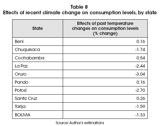
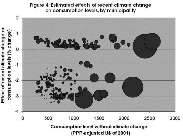
<body><![CDATA[<p align="justify"><font size="2" face="Verdana, Arial, Helvetica, sans-serif">  As there has been no systematic change in  precipitation, the precipitation terms cancel   out, and the other factors, education and urbanization  rates, we will maintain constant, so as    <br>   to isolate the climate change effect. Thus the ratio  of Climate Change Consumption to No   Climate Change Consumption can be written as:</font></p>     <p align="center"><font size="2" face="Verdana, Arial, Helvetica, sans-serif"><img src="/img/revistas/rlde/n22/a03_ecuacion_02.gif" width="489" height="77"></font></p>     <p align="justify"><font size="2" face="Verdana, Arial, Helvetica, sans-serif">  After estimating this ratio for each municipality, it  is straightforward to calculate the   percentage change in consumption levels that can be  attributed to climate change. At the   national level, the model estimates that climate  change during the last 50 years has caused a   reduction in consumption of about 1.3%.</font></p>     <p align="justify"><font size="2" face="Verdana, Arial, Helvetica, sans-serif"><a href="#t8"> Table 8</a> shows the results disaggregated at the state  level. The most disadvantaged states   are the highland states Oruro, Potos&iacute; and La Paz,  which are estimated to have lost almost 3%   of their consumption capacity due to the already cold  climates becoming colder. Chuquisaca   and Tarija have also lost out according to this  simulation, but a bit less, as they were initially   warmer, and the slope of the temperature/consumption  relationship was thus less steep. All   lowland states have gained slightly.</font></p>     <p align="justify"><a name="t8" id="t8"></a></p>     <p align="center"><img src="/img/revistas/rlde/n22/a03_table_08.gif" width="519" height="405"></p>     <p align="justify"><a href="#f4"><font size="2" face="Verdana, Arial, Helvetica, sans-serif"> Figure 4</font></a><font size="2" face="Verdana, Arial, Helvetica, sans-serif"> shows the estimated effects of recent climate  change on <i>per  capita </i>consumption   levels in all 311 municipalities. The municipalities  are grouped in winners and losers, with   no municipality being entirely unaffected. The winners  are all lowland municipalities,   representing 51% of the population. The losers are all  highland municipalities, representing   about 49% of the Bolivian population.</font></p>     <p align="justify"><a name="f4"></a></p>     <p align="center"><img src="/img/revistas/rlde/n22/a03_figure_04.gif" width="602" height="452"></p>     ]]></body>

<body><![CDATA[<p align="justify"><font size="2" face="Verdana, Arial, Helvetica, sans-serif">  There is a weak but statistically significant positive  relationship (&rho; = 0.28) between initial   level of consumption and the estimated effects of past  climate change. This suggests that it   is generally the poorest municipalities which have  experienced the most negative effects of   recent climate change, implying that recent climate  change has contributed to an increase in   both poverty and inequality.</font></p>     <p align="justify"><font size="2" face="Verdana, Arial, Helvetica, sans-serif">  The poor highland municipalities, which are most  adversely affected, also happen to have   much larger proportions of indigenous populations than  the lowland municipalities which   have benefitted from recent climate change. This  implies that the indigenous people of Bolivia   are on average more adversely affected from recent  climate change than the non-indigenous population, simply because they happen to live in  areas where the climate has turned less   beneficial for human development (colder).</font></p>     <p align="justify">&nbsp;</p>     <p align="justify"><font size="3" face="Verdana, Arial, Helvetica, sans-serif"><b>6. Conclusions</b></font></p>     <p align="justify"><font size="2" face="Verdana, Arial, Helvetica, sans-serif">  This paper has analyzed the direct evidence of climate  change in Bolivia over the last 60   years. Contrary to expectations, and contrary to the  predictions of most General Circulation   models, this evidence shows a consistent cooling trend  of about 0.2&ordm;C per decade over   all highland areas, and only slight, scattered evidence  of warming in the lowland areas. No   systematic trends in precipitation were detected, only  decade-long cycles. There are indications   that the decrease in average temperatures in the  highlands is hiding an increase in daytime and   summer temperatures but a decrease in nighttime and  winter temperatures, although much   more detailed daily temperature records would be  needed to confirm this.</font></p>     <p align="justify"><font size="2" face="Verdana, Arial, Helvetica, sans-serif">  Using municipality level data, models of the  relationships between climate, life expectancy   and consumption levels were estimated (controlling for  other factors that might affect life   expectancy and consumption levels). The results  suggest that consumption possibilities in   Bolivia increase with temperature, but at a decreasing  rate. Consumption levels are almost   twice as large in the warmest parts of Bolivia  compared to the coldest parts (when controlling   for differences in education levels, urbanization  rates, and precipitation). Precipitation,   however, was not found to have any systematic effect  on consumption levels. Neither   temperature nor precipitation was found to have any  systematic effects on life expectancy.</font></p>     <p align="justify"><font size="2" face="Verdana, Arial, Helvetica, sans-serif">  When simulating the impact of recent climate change in  Bolivia (1&ordm;C reduction in   temperatures in the already cold highlands, and a  0.25&ordm;C increase in temperatures in   the already hot lowlands over the last 50 years), we  found an adverse impact on national   consumption levels of 1.3%. Since the predominantly  poor and indigenous population in the   highlands experienced a negative effect due to recent  cooling and the much richer population   in the lowlands experienced slightly positive effects  of modest warming, the overall effect of   recent climate change would be an increase in  inequality between Bolivian municipalities and   an increase in poverty.</font></p>     <p align="justify"><font size="2" face="Verdana, Arial, Helvetica, sans-serif">  Notice that this is due to the direction of recent  climate changes in Bolivia, and not due to   any inherent characteristics of the poor which might  make them more vulnerable to climate   change. If recent climate change had showed warming  across the country (as climate models typically suggest), then the poor in the highlands  would have benefited much more than the rich in the lowlands, thus reducing poverty and  inequality.</font></p>     <p align="justify"><font size="2" face="Verdana, Arial, Helvetica, sans-serif">  The magnitudes of the estimated impacts are not large,  however. A reduction in   consumption levels of 3-4% (the most adverse effects  encountered) over a 50 year period   corresponds to just one year of low growth.</font></p>     <p align="justify"><font size="2" face="Verdana, Arial, Helvetica, sans-serif">  It is important to keep in mind that the approach of  this paper is designed to capture the   long term effects of climate change, <i>after </i>people have adjusted to the  changed climate. The paper   does not address transition costs and costs of normal  climate variability. This is a reasonable   approach if climate change takes place slowly and  predictably, so that people can gradually   adjust their behaviors (for example, by sowing a  different crop than their parents used to). It is   assumed that people base their economic decisions on  what their current climate is like, rather   than on what the climate was like a generation ago,  just as they should base their economic   decisions on current market conditions rather than on  market conditions 30 years earlier.</font></p>     ]]></body>
<body><![CDATA[<p align="justify"><font size="2" face="Verdana, Arial, Helvetica, sans-serif">  It is also assumed that for any given  temperature-precipitation combination, climate has   not become more unpredictable. At the aggregate level,  however, predictability may have   changed, since there are now more municipalities with  lower temperatures. Places where   temperatures oscillate close to the freezing point  inherently have more unpredictable weather   than places which are consistently hot and humid, and  temperature variations close to zero   have more severe consequences. Indeed, we find that  the two highland stations, Oruro and   Chara&ntilde;a, have experienced increased variability in  temperatures. But the rest of the stations   have experienced no significant changes in variability  or even reduced variability. With respect   to precipitation, we found three stations (Cobija,  Yacuiba and San Javier) that had higher   precipitation variability since 1991 compared to the  reference period 1960-90. The rest had   either lower or unchanged variability.</font></p>     <p align="justify"><font size="2" face="Verdana, Arial, Helvetica, sans-serif">  The modest impacts of climate <i>change </i>(the slow, systematic changes in  average temperature   and precipitation) do not preclude large impacts from  climate <i>variability</i>. Indeed many studies   have evaluated the costs of El Ni&ntilde;o and La Ni&ntilde;a events  in Bolivia (causing extreme droughts   and flooding) finding costs of up to 18% of annual GDP  for the 1982-83 El Ni&ntilde;o event; 7%   for the 1997-98 El Ni&ntilde;o; 4.2% from the 2006-2007 El  Ni&ntilde;o; and 3.4% from the 2007-2008 La   Ni&ntilde;a event (Bolivia 2004; CAF 2000; CEPAL 2007 and  2008).</font></p>     <p align="justify"><font size="2" face="Verdana, Arial, Helvetica, sans-serif"><b>Predicting the effects of future climate change</b></font></p>     <p align="justify"><font size="2" face="Verdana, Arial, Helvetica, sans-serif">  While recent climate change can be analyzed and documented  using temperature and   precipitation records from weather stations spread  across the national territory, it is much   more difficult to assess the impacts of future climate  change, because there is very little   scientific consensus about how the local climates in  Bolivia are going to change in the future.</font></p>     <p align="justify"><font size="2" face="Verdana, Arial, Helvetica, sans-serif">  The Intergovernmental Panel on Climate Change uses a  combination of different General   Circulation Models to predict future climates. For  some regions these models do a reasonably   good job at replicating past climate change and  current climatic conditions, and there is a high   level of agreement between the many different models.  This is not the case for South America   in general, and even less the case for Bolivia. Not a  single model has replicated the recent   temperature reductions observed across most of  Bolivia. According to the IPCC4, Working   Group I chapter on Regional Climate Projections for  Latin America:</font></p>     <blockquote>       <p align="justify"><font size="2" face="Verdana, Arial, Helvetica, sans-serif">  The systematic errors in simulating current mean  tropical climate and its variability and the     large inter-model differences in future changes in El  Ni&ntilde;o amplitude preclude a conclusive     assessment of the regional changes over large areas of  Central and South America. (&hellip;)    <br>     The high and sharp Andes Mountains are unresolved in  low resolution models, affecting     the assessment over much of the continent (Christensen <i>et al.</i>, 2007).</font></p> </blockquote>     <p align="justify"><font size="2" face="Verdana, Arial, Helvetica, sans-serif">  Despite this uncertainty, the IPCC report finds it  very likely that temperatures will increase   over all areas of South America over the rest of this  century. If this turns out to be true, the   recent cooling trend would be reverted, and the  climate in Bolivia might return to &ldquo;normal&rdquo;   (the 1961-90 average) within the next 2-3 decades.</font></p>     <p align="justify"><font size="2" face="Verdana, Arial, Helvetica, sans-serif">  However, &ldquo;normal&rdquo; climate in Bolivia includes  tremendous climate variability with either   El Ni&ntilde;o or La Ni&ntilde;a conditions almost every year. If  each of these events causes losses of 3-4%    ]]></body>
<body><![CDATA[<br>   of GDP, they make all the difference between a country  growing steadily towards prosperity   and a country permanently stuck in poverty.  Vulnerability has clearly been reduced since    <br>   the devastating El Ni&ntilde;o episode of 1982-83, but  further steps to reduce vulnerability are still   necessary.</font></p>     <p align="justify">&nbsp;</p>     <p align="right"><font size="2" face="Verdana, Arial, Helvetica, sans-serif"><i><b>Art&iacute;culo  recibido en:</b> 20 de junio de 2009</i>    <br>   <i><b>Manejado  por:</b> ABCE</i>    <br>   <i><b>Aceptado  en:</b> 18 de septiembre de 2014</i>    <br>   </font></p>     <p><font size="3"><b><font face="Verdana, Arial, Helvetica, sans-serif">References</font></b><font face="Verdana, Arial, Helvetica, sans-serif"></font></font></p>     <p align="justify"><font size="2" face="Verdana, Arial, Helvetica, sans-serif">  1. Andersen, L. E. &amp; D. Verner (2009). &ldquo;Social  Impacts of Climate Change in Chile: A   municipal level analysis of the effects of recent and  future climate change on human   development and inequality, Draft, February.</font></p>     <p align="justify"><font size="2" face="Verdana, Arial, Helvetica, sans-serif">  2. Andersen, L. E., A. Suxo &amp; D. Verner (2009). &ldquo;Social  Impacts of Climate Change in   Peru: A district level analysis of the effects of  recent and future climate change on human   development and inequality, Draft, February.</font></p>     ]]></body>
<body><![CDATA[<p align="justify"><font size="2" face="Verdana, Arial, Helvetica, sans-serif"> 3. Andersen, L. E., S. Rom&aacute;n &amp; D. Verner (2009). &ldquo;Social  Impacts of Climate Change in   Brazil: A municipal level analysis of the effects of  recent and future climate change on   human development and inequality, Draft, February.</font></p>     <p align="justify"><font size="2" face="Verdana, Arial, Helvetica, sans-serif">  4.  Bolivia (2004) &ldquo;La gesti&oacute;n del riesgo en Bolivia.&rdquo; Ministerio de Defensa Nacional de   Bolivia.</font></p>     <p align="justify"><font size="2" face="Verdana, Arial, Helvetica, sans-serif">  5. Brown, Lawrence A. &amp; John Paul Jones III  (1985). &ldquo;Spatial Variation in Migration   Processes and Development: A Costa Rican Example of  Conventional Modeling   Augmented by the Expansion Method.&rdquo; <i>Demography</i>, 22(3), 327-352.</font></p>     <p align="justify"><font size="2" face="Verdana, Arial, Helvetica, sans-serif">  6.  CAF (2000) &ldquo;Las lecciones de El Ni&ntilde;o &ndash; Bolivia.&rdquo; Corporaci&oacute;n Andina de Fomento,   Caracas,  Venezuela</font></p>     <p align="justify"><font size="2" face="Verdana, Arial, Helvetica, sans-serif">  7.  CEPAL (2007). &ldquo;Informe sobre el impacto del fen&oacute;meno de El Ni&ntilde;o en Bolivia.&rdquo;   Comisi&oacute;n  Econ&oacute;mica para Am&eacute;rica Latina y El Caribe, April.</font></p>     <p align="justify"><font size="2" face="Verdana, Arial, Helvetica, sans-serif">  8.  CEPAL (2008). &ldquo;Informe sobre el impacto del fen&oacute;meno de La Ni&ntilde;a en Bolivia.&rdquo;   Comisi&oacute;n  Econ&oacute;mica para Am&eacute;rica Latina y El Caribe, April.</font></p>     <p align="justify"><font size="2" face="Verdana, Arial, Helvetica, sans-serif">  9. Christensen, J.H., B. Hewitson, A. Busuioc, A.  Chen, X. Gao, I. Held, R. Jones, R.K. Kolli,   W.-T. Kwon, R. Laprise, V. Maga&ntilde;a Rueda, L. Mearns,  C.G. Men&eacute;ndez, J. R&auml;is&auml;nen, A.   Rinke, A. Sarr and P. Whetton (2007). &ldquo;Regional  Climate Projections.&rdquo; In: S. Solomon,   D. Qin, M. Manning, Z. Chen, M. Marquis, K.B. Averyt,  M. Tignor and H.L. Miller   (eds.), <i>Climate Change 2007: The Physical Science Basis.  Contribution of Working Group I to the Fourth Assessment  Report of the Intergovernmental Panel on Climate Change</i>. Cambridge   University Press, Cambridge, United Kingdom and New  York, NY, USA.</font></p>     <p align="justify"><font size="2" face="Verdana, Arial, Helvetica, sans-serif">  10. Francou, B., E. Ramirez, B. Caceres &amp; J.  Mendoza (2000). &ldquo;Glacier  evolution in the   Tropical Andes during the last decades of the 20th  Century: Chacaltaya, Bolivia, and   Antizana,  Ecuador.&rdquo; <i>Ambio</i>,  29(7): 416 -422.</font></p>     <p align="justify"><font size="2" face="Verdana, Arial, Helvetica, sans-serif">  11.  Gonzales Iwanciw, J., J. Cusicanqui Giles &amp; M. Aparicio Effen (n.d.). &ldquo;Vulnerabilidad  y   adaptaci&oacute;n  al cambio Clim&aacute;tico en las regiones del Lago Titicaca y los valles cruce&ntilde;os   de  Bolivia: sistematizaci&oacute;n de los resultados de la investigaci&oacute;n participativa,  consultas   y  estudios de caso.&rdquo; Ministerio de Planificaci&oacute;n del Desarrollo, Programa  Nacional de   Cambios  Clim&aacute;ticos, Bolivia.</font></p>     <p align="justify"><font size="2" face="Verdana, Arial, Helvetica, sans-serif">  12.  Hoffmann, G., E. Ramirez, J. D. Taupin, B. Francou, P. Ribstein, R. Delmas, H.  D&uuml;rr,   R.  Gallaire, J. Sim&otilde;es, U. Schotterer, M. Stievenard &amp; M. Werner (2003). &ldquo;Coherent   isotope history of Andean ice cores over the last  century.&rdquo; <i>Geophysical  Research Letters</i>,   30(4): 1179-1182.</font></p>     ]]></body>
<body><![CDATA[<p align="justify"><font size="2" face="Verdana, Arial, Helvetica, sans-serif">  13. Horowitz, J. K. (2006). &ldquo;The Income-Temperature  Relationship in a Cross-Section of   Countries and its Implications for Global Warming.&rdquo;  Department of Agricultural and   Resource Economics, University of Maryland, Submitted  manuscript, July. Available in:   <a href="http://faculty.arec.umd.edu/jhorowitz/Income-Temp-i.pdf" target="_blank">http://faculty.arec.umd.edu/jhorowitz/Income-Temp-i.pdf</a></font></p>     <p align="justify"><font size="2" face="Verdana, Arial, Helvetica, sans-serif">  14. Masters, W. A. &amp; M. S. McMillan (2001). &ldquo;Climate  and Scale in Economic Growth,&rdquo;   <i>Journal of Economic Growth</i>, 6(3): 167-186.</font></p>     <p align="justify"><font size="2" face="Verdana, Arial, Helvetica, sans-serif">  15. Mendelsohn, R., W. Nordhaus &amp; D. Shaw (1994). &ldquo;The  Impact of Global Warming on   Agriculture: A Ricardian Analysis,&rdquo; <i>American Economic Review</i>, 84(4): 753-71.</font></p>     <!-- ref --><p align="justify"><font size="2" face="Verdana, Arial, Helvetica, sans-serif">  16.  PNUD (2004). &Iacute;ndice de <i>Desarrollo Humano en los  municipios de Bolivia. </i>Informe   Nacional  de Desarrollo Humano 2004, La Paz, Bolivia.</font>&nbsp;&nbsp;&nbsp;&nbsp;&nbsp;&nbsp;&nbsp;&nbsp;[&#160;<a href="javascript:void(0);" onclick="javascript: window.open('/scielo.php?script=sci_nlinks&ref=522715&pid=S2074-4706201400020000300016&lng=','','width=640,height=500,resizable=yes,scrollbars=1,menubar=yes,');">Links</a>&#160;]<!-- end-ref --><p align="justify"><font size="2" face="Verdana, Arial, Helvetica, sans-serif">  17.  Quiggin, J. &amp; J. K. Horowitz (1999). &ldquo;The Impact of Global Warming on Agriculture: A   Ricardian Analysis: Comment,&rdquo; <i>American Economic Review</i>, 89(4): 1044-45.</font></p>     <p align="justify"><font size="2" face="Verdana, Arial, Helvetica, sans-serif">  18.  Ram&iacute;rez, E. (2008). &ldquo;Impactos del cambio  clim&aacute;tico y gesti&oacute;n del agua sobre la   disponibilidad  de recursos h&iacute;dricos para las ciudades de La Paz y El Alto.&rdquo; <i>Revista Virtual REDESMA</i>, 2(3): 49-61.</font></p>     <p align="justify"><font size="2" face="Verdana, Arial, Helvetica, sans-serif">  19.  Ram&iacute;rez, E., B. Francou,  P. Ribstein, M. Descloitres, R. Guerin, J. Mendoza, R. Gallaire,   B.  Pouyaud, &amp; E. Jordan (2001). &ldquo;Small glaciers disappearing in the tropical Andes.   A case study in Bolivia: Glaciar Chacaltaya (16&deg;S).&rdquo; <i>Journal of Glaciology, </i>47(157):   187-194.</font></p>     <p align="justify"><font size="2" face="Verdana, Arial, Helvetica, sans-serif">  20. Tol, R. S. J. (2005) &ldquo;Emission abatement versus  development as strategies to reduce   vulnerability to climate change: an application of  FUND.&rdquo; <i>Environment  and Development Economics</i>, 10: 615-629.</font></p>     <p align="justify"><font size="2" face="Verdana, Arial, Helvetica, sans-serif">  21. Trenberth, K.E., P.D. Jones, P. Ambenje, R.  Bojariu, D. Easterling, A. Klein Tank, D.   Parker, F. Rahimzadeh, J.A. Renwick, M. Rusticucci, B.  Soden and P. Zhai (2007).  &ldquo;Observations: Surface and Atmospheric Climate Change.&rdquo;  In: S. Solomon, D. Qin, M.   Manning, Z. Chen, M. Marquis, K.B. Averyt, M. Tignor  and H.L. Miller (eds.) <i>Climate Change 2007: The Physical  Science Basis. Contribution of Working Group I to the Fourth assessment Report of the  Intergovernmental Panel on Climate Change. </i>Cambridge  University Press,  Cambridge, United Kingdom and New York, NY, USA.</font></p>     <p align="justify">&nbsp;</p>     ]]></body>
<body><![CDATA[<p><b><font face="Verdana, Arial, Helvetica, sans-serif" size="3">Annex:</font></b></p>     <p><b><font face="Verdana, Arial, Helvetica, sans-serif" size="2">Monthly temperature and precipitation anomalies</font></b></p>     <p align="center"><img src="/img/revistas/rlde/n22/a03_x01_01.gif" width="904" height="618"></p>     <p align="center">&nbsp;</p>     <p align="center"><img src="/img/revistas/rlde/n22/a03_x01_02.gif" width="917" height="596"></p>     <p align="center">&nbsp;</p>     <p align="center"><img src="/img/revistas/rlde/n22/a03_x01_03.gif" width="904" height="583"></p>     <p align="center">&nbsp;</p>     <p align="center"><img src="/img/revistas/rlde/n22/a03_x01_04.gif" width="907" height="584"></p>     <p align="center">&nbsp;</p>     ]]></body>
<body><![CDATA[<p align="center"><img src="/img/revistas/rlde/n22/a03_x01_05.gif" width="906" height="312"></p>     <p align="center">&nbsp;</p>     <p align="center">&nbsp;</p>     <p align="center"><img src="/img/revistas/rlde/n22/a03_x02_01.gif" width="914" height="631"></p>     <p align="center">&nbsp;</p>     <p align="center"><img src="/img/revistas/rlde/n22/a03_x02_02.gif" width="904" height="592"></p>     <p align="center">&nbsp;</p>     <p align="center"><img src="/img/revistas/rlde/n22/a03_x02_03.gif" width="912" height="585"></p>     <p align="center">&nbsp;</p>     <p align="center"><img src="/img/revistas/rlde/n22/a03_x02_04.gif" width="907" height="584"></p>     ]]></body>
<body><![CDATA[<p align="center">&nbsp;</p>     <p align="center"><img src="/img/revistas/rlde/n22/a03_x02_05.gif" width="913" height="613">    <br> </p>     <p><b><font face="Verdana, Arial, Helvetica, sans-serif" size="3">Notas</font></b></p>     <p>*<font size="2" face="Verdana, Arial, Helvetica, sans-serif"> Institute for Advanced Development Studies (INESAD) and Universidad Privada Boliviana (UPB), La Paz, Bolivia.    <br>       <b>Contact:</b> <a href="mailto:landersen@inesad.edu.bo">landersen@inesad.edu.bo</a></font></p>     <p><font size="2" face="Verdana, Arial, Helvetica, sans-serif"> ** Office of Evaluation and Oversight, Inter-American Development Bank, Washington D.C.    <br>       <b>Contact:</b> <a href="mailto:DORTEV@iadb.org">DORTEV@iadb.org</a></font>.</p>     <p align="justify"><font size="2" face="Verdana, Arial, Helvetica, sans-serif">1 This paper forms part of the World Bank research project &ldquo;Social Impacts of Climate Change and Environmental    Degradation in the LAC Region.&rdquo; The authors greatly appreciate the comments, uggestions and inputs received   from Pablo Fajnzylber, Kirk Hamilton, Jacoby Hanan, Jens Hesselbjerg Christensen, Jakob Kronik, Andrea Liverani,   Joergen Eivind Olesen, Claus P&ouml;rtner, Tine Rossing, Olivier Rubin, Emmanuel Skoufias, Fabi&aacute;n Soria and Addy   Suxo. The findings, interpretations and conclusions expressed in this paper are those of the authors and do not   necessarily reflect the views of the Executive Directors of The World Bank or the governments they represent.</font></p>     <p align="justify"><font size="2" face="Verdana, Arial, Helvetica, sans-serif">2 This data is available for free at <a href="http://www7.ncdc.noaa.gov/IPS/mcdw/mcdw.html" target="_blank">http://www7.ncdc.noaa.gov/IPS/mcdw/mcdw.html</a>.</font></p>     ]]></body>
<body><![CDATA[<p align="justify"><font size="2" face="Verdana, Arial, Helvetica, sans-serif">3 However,  this decrease is not considered unusual in a historical context and over the  whole 20th century the   isotope index  is stable</font></p>     <p align="justify"><font size="2" face="Verdana, Arial, Helvetica, sans-serif"> 4 According  to NASA&rsquo;s International Satellite Cloud Climatology Project &ndash; ISCCP  (<a href="http://isccp.giss.nasa.gov/index.html" target="_blank">http://isccp.giss.nasa.gov/index.html</a>),  average tropical cloud cover has decreased from about 66% in the 1980s to about  61% in the first 8 years   of this  century.</font></p>     <p align="justify">&nbsp;</p>      ]]></body><back>
<ref-list>
<ref id="B1">
<label>1</label><nlm-citation citation-type="">
<person-group person-group-type="author">
<name>
<surname><![CDATA[Andersen]]></surname>
<given-names><![CDATA[L.E.]]></given-names>
</name>
<name>
<surname><![CDATA[Verner]]></surname>
<given-names><![CDATA[D.]]></given-names>
</name>
</person-group>
<source><![CDATA[Social Impacts of Climate Change in Chile: A municipal level analysis of the effects of recent and future climate change on human development and inequality]]></source>
<year>2009</year>
</nlm-citation>
</ref>
<ref id="B2">
<label>2</label><nlm-citation citation-type="">
<person-group person-group-type="author">
<name>
<surname><![CDATA[Andersen]]></surname>
<given-names><![CDATA[L.E.]]></given-names>
</name>
<name>
<surname><![CDATA[Suxo]]></surname>
<given-names><![CDATA[A.]]></given-names>
</name>
<name>
<surname><![CDATA[Verner]]></surname>
<given-names><![CDATA[D.]]></given-names>
</name>
</person-group>
<source><![CDATA[Social Impacts of Climate Change in Peru: A district level analysis of the effects of recent and future climate change on human development and inequality]]></source>
<year>2009</year>
</nlm-citation>
</ref>
<ref id="B3">
<label>3</label><nlm-citation citation-type="">
<person-group person-group-type="author">
<name>
<surname><![CDATA[Andersen]]></surname>
<given-names><![CDATA[L.E.]]></given-names>
</name>
<name>
<surname><![CDATA[Román]]></surname>
<given-names><![CDATA[S.]]></given-names>
</name>
<name>
<surname><![CDATA[Verner]]></surname>
<given-names><![CDATA[D.]]></given-names>
</name>
</person-group>
<source><![CDATA[Social Impacts of Climate Change in Brazil: A municipal level analysis of the effects of recent and future climate change on human development and inequality]]></source>
<year>2009</year>
</nlm-citation>
</ref>
<ref id="B4">
<label>4</label><nlm-citation citation-type="book">
<collab>Bolivia</collab>
<source><![CDATA[La gestión del riesgo en Bolivia]]></source>
<year>2004</year>
<publisher-loc><![CDATA[X ]]></publisher-loc>
<publisher-name><![CDATA[Ministerio de Defensa Nacional de Bolivia]]></publisher-name>
</nlm-citation>
</ref>
<ref id="B5">
<label>5</label><nlm-citation citation-type="journal">
<person-group person-group-type="author">
<name>
<surname><![CDATA[Brown]]></surname>
<given-names><![CDATA[Lawrence A.]]></given-names>
</name>
<name>
<surname><![CDATA[Jones III]]></surname>
<given-names><![CDATA[John Paul]]></given-names>
</name>
</person-group>
<article-title xml:lang="en"><![CDATA[Spatial Variation in Migration Processes and Development: A Costa Rican Example of Conventional Modeling Augmented by the Expansion Method]]></article-title>
<source><![CDATA[Demography]]></source>
<year>1985</year>
<volume>22</volume>
<numero>3</numero>
<issue>3</issue>
<page-range>327-352</page-range></nlm-citation>
</ref>
<ref id="B6">
<label>6</label><nlm-citation citation-type="book">
<collab>CAF</collab>
<source><![CDATA[Las lecciones de El Niño - Bolivia]]></source>
<year>2000</year>
<publisher-loc><![CDATA[Caracas ]]></publisher-loc>
<publisher-name><![CDATA[Corporación Andina de Fomento]]></publisher-name>
</nlm-citation>
</ref>
<ref id="B7">
<label>7</label><nlm-citation citation-type="">
<collab>CEPAL</collab>
<source><![CDATA[Informe sobre el impacto del fenómeno de El Niño en Bolivia]]></source>
<year>2007</year>
<month> A</month>
<day>pr</day>
<publisher-loc><![CDATA[Comisión Económica para América Latina y El Caribe ]]></publisher-loc>
</nlm-citation>
</ref>
<ref id="B8">
<label>8</label><nlm-citation citation-type="book">
<collab>CEPAL</collab>
<source><![CDATA[Informe sobre el impacto del fenómeno de La Niña en Bolivia]]></source>
<year>2008</year>
<month> A</month>
<day>pr</day>
<publisher-loc><![CDATA[X ]]></publisher-loc>
<publisher-name><![CDATA[Comisión Económica para América Latina y El Caribe]]></publisher-name>
</nlm-citation>
</ref>
<ref id="B9">
<label>9</label><nlm-citation citation-type="book">
<person-group person-group-type="author">
<name>
<surname><![CDATA[Christensen]]></surname>
<given-names><![CDATA[J.H.]]></given-names>
</name>
<name>
<surname><![CDATA[Hewitson]]></surname>
<given-names><![CDATA[B.]]></given-names>
</name>
<name>
<surname><![CDATA[Busuioc]]></surname>
<given-names><![CDATA[A.]]></given-names>
</name>
<name>
<surname><![CDATA[Chen]]></surname>
<given-names><![CDATA[A.]]></given-names>
</name>
<name>
<surname><![CDATA[Gao]]></surname>
<given-names><![CDATA[X.]]></given-names>
</name>
<name>
<surname><![CDATA[Held]]></surname>
<given-names><![CDATA[I.]]></given-names>
</name>
<name>
<surname><![CDATA[Jones]]></surname>
<given-names><![CDATA[R.]]></given-names>
</name>
<name>
<surname><![CDATA[Kolli]]></surname>
<given-names><![CDATA[R.K.]]></given-names>
</name>
<name>
<surname><![CDATA[Kwon]]></surname>
<given-names><![CDATA[W.-T.]]></given-names>
</name>
<name>
<surname><![CDATA[Laprise]]></surname>
<given-names><![CDATA[R.]]></given-names>
</name>
<name>
<surname><![CDATA[Magaña Rueda]]></surname>
<given-names><![CDATA[V.]]></given-names>
</name>
<name>
<surname><![CDATA[Mearns]]></surname>
<given-names><![CDATA[L.]]></given-names>
</name>
<name>
<surname><![CDATA[Menéndez]]></surname>
<given-names><![CDATA[C.G.]]></given-names>
</name>
<name>
<surname><![CDATA[Räisänen]]></surname>
<given-names><![CDATA[J.]]></given-names>
</name>
<name>
<surname><![CDATA[Rinke]]></surname>
<given-names><![CDATA[A.]]></given-names>
</name>
<name>
<surname><![CDATA[Sarr]]></surname>
<given-names><![CDATA[A.]]></given-names>
</name>
<name>
<surname><![CDATA[Whetton]]></surname>
<given-names><![CDATA[P.]]></given-names>
</name>
</person-group>
<article-title xml:lang="en"><![CDATA[Regional Climate Projections]]></article-title>
<person-group person-group-type="editor">
<name>
<surname><![CDATA[Solomon]]></surname>
<given-names><![CDATA[S.]]></given-names>
</name>
<name>
<surname><![CDATA[Qin]]></surname>
<given-names><![CDATA[D.]]></given-names>
</name>
<name>
<surname><![CDATA[Manning]]></surname>
<given-names><![CDATA[M.]]></given-names>
</name>
<name>
<surname><![CDATA[Chen]]></surname>
<given-names><![CDATA[Z.]]></given-names>
</name>
<name>
<surname><![CDATA[Marquis]]></surname>
<given-names><![CDATA[M.]]></given-names>
</name>
<name>
<surname><![CDATA[Averyt]]></surname>
<given-names><![CDATA[K.B.]]></given-names>
</name>
<name>
<surname><![CDATA[Tignor]]></surname>
<given-names><![CDATA[M.]]></given-names>
</name>
<name>
<surname><![CDATA[Miller]]></surname>
<given-names><![CDATA[H.L.]]></given-names>
</name>
</person-group>
<source><![CDATA[Climate Change 2007: The Physical Science Basis. Contribution of Working Group I to the Fourth Assessment Report of the Intergovernmental Panel on Climate Change]]></source>
<year>2007</year>
<publisher-loc><![CDATA[Cambridge, New York^eNY NY]]></publisher-loc>
<publisher-name><![CDATA[Cambridge University Press]]></publisher-name>
</nlm-citation>
</ref>
<ref id="B10">
<label>10</label><nlm-citation citation-type="journal">
<person-group person-group-type="author">
<name>
<surname><![CDATA[Francou]]></surname>
<given-names><![CDATA[B.]]></given-names>
</name>
<name>
<surname><![CDATA[Ramirez]]></surname>
<given-names><![CDATA[E.]]></given-names>
</name>
<name>
<surname><![CDATA[Caceres]]></surname>
<given-names><![CDATA[B.]]></given-names>
</name>
<name>
<surname><![CDATA[Mendoza]]></surname>
<given-names><![CDATA[J.]]></given-names>
</name>
</person-group>
<article-title xml:lang="en"><![CDATA[Glacier evolution in the Tropical Andes during the last decades of the 20th Century: Chacaltaya, Bolivia, and Antizana, Ecuador]]></article-title>
<source><![CDATA[Ambio]]></source>
<year>2000</year>
<volume>29</volume>
<numero>7</numero>
<issue>7</issue>
<page-range>416 -422</page-range></nlm-citation>
</ref>
<ref id="B11">
<label>11</label><nlm-citation citation-type="book">
<person-group person-group-type="author">
<name>
<surname><![CDATA[Gonzales Iwanciw]]></surname>
<given-names><![CDATA[J.]]></given-names>
</name>
<name>
<surname><![CDATA[Cusicanqui Giles]]></surname>
<given-names><![CDATA[J.]]></given-names>
</name>
<name>
<surname><![CDATA[Aparicio Effen]]></surname>
<given-names><![CDATA[M.]]></given-names>
</name>
</person-group>
<source><![CDATA[Vulnerabilidad y adaptación al cambio Climático en las regiones del Lago Titicaca y los valles cruceños de Bolivia: sistematización de los resultados de la investigación participativa, consultas y estudios de caso]]></source>
<year></year>
<publisher-name><![CDATA[Ministerio de Planificación del Desarrollo, Programa Nacional de Cambios Climáticos, Bolivia]]></publisher-name>
</nlm-citation>
</ref>
<ref id="B12">
<label>12</label><nlm-citation citation-type="journal">
<person-group person-group-type="author">
<name>
<surname><![CDATA[Hoffmann]]></surname>
<given-names><![CDATA[G.]]></given-names>
</name>
<name>
<surname><![CDATA[Ramirez]]></surname>
<given-names><![CDATA[E.]]></given-names>
</name>
<name>
<surname><![CDATA[Taupin]]></surname>
<given-names><![CDATA[J.D. Francou]]></given-names>
</name>
<name>
<surname><![CDATA[B.]]></surname>
<given-names><![CDATA[Ribstein]]></given-names>
</name>
<name>
<surname><![CDATA[P.]]></surname>
<given-names><![CDATA[Delmas]]></given-names>
</name>
<name>
<surname><![CDATA[R.]]></surname>
<given-names><![CDATA[Dürr]]></given-names>
</name>
<name>
<surname><![CDATA[H. Gallaire]]></surname>
<given-names><![CDATA[R.]]></given-names>
</name>
<name>
<surname><![CDATA[Simões]]></surname>
<given-names><![CDATA[J.]]></given-names>
</name>
<name>
<surname><![CDATA[Schotterer]]></surname>
<given-names><![CDATA[U.]]></given-names>
</name>
<name>
<surname><![CDATA[Stievenard]]></surname>
<given-names><![CDATA[M.]]></given-names>
</name>
<name>
<surname><![CDATA[Werner]]></surname>
<given-names><![CDATA[M.]]></given-names>
</name>
</person-group>
<article-title xml:lang="en"><![CDATA[Coherent isotope history of Andean ice cores over the last century]]></article-title>
<source><![CDATA[Geophysical Research Letters]]></source>
<year>2003</year>
<volume>30</volume>
<numero>4</numero>
<issue>4</issue>
<page-range>1179-1182</page-range></nlm-citation>
</ref>
<ref id="B13">
<label>13</label><nlm-citation citation-type="book">
<person-group person-group-type="author">
<name>
<surname><![CDATA[Horowitz]]></surname>
<given-names><![CDATA[J.K.]]></given-names>
</name>
</person-group>
<source><![CDATA[The Income-Temperature Relationship in a Cross-Section of Countries and its Implications for Global Warming]]></source>
<year>2006</year>
<publisher-name><![CDATA[Department of Agricultural and Resource Economics, University of Maryland]]></publisher-name>
</nlm-citation>
</ref>
<ref id="B14">
<label>14</label><nlm-citation citation-type="journal">
<person-group person-group-type="author">
<name>
<surname><![CDATA[Masters]]></surname>
<given-names><![CDATA[W.A.]]></given-names>
</name>
<name>
<surname><![CDATA[McMillan]]></surname>
<given-names><![CDATA[M.S.]]></given-names>
</name>
</person-group>
<article-title xml:lang="en"><![CDATA[Climate and Scale in Economic Growth]]></article-title>
<source><![CDATA[Journal of Economic Growth]]></source>
<year>2001</year>
<volume>6</volume>
<numero>3</numero>
<issue>3</issue>
<page-range>167-186</page-range></nlm-citation>
</ref>
<ref id="B15">
<label>15</label><nlm-citation citation-type="journal">
<person-group person-group-type="author">
<name>
<surname><![CDATA[Mendelsohn]]></surname>
<given-names><![CDATA[R.]]></given-names>
</name>
<name>
<surname><![CDATA[Nordhaus]]></surname>
<given-names><![CDATA[W]]></given-names>
</name>
<name>
<surname><![CDATA[Shaw]]></surname>
<given-names><![CDATA[D.]]></given-names>
</name>
</person-group>
<article-title xml:lang="en"><![CDATA[The Impact of Global Warming on Agriculture: A Ricardian Analysis]]></article-title>
<source><![CDATA[American Economic Review]]></source>
<year>1994</year>
<volume>84</volume>
<numero>4</numero>
<issue>4</issue>
<page-range>753-71</page-range></nlm-citation>
</ref>
<ref id="B16">
<label>16</label><nlm-citation citation-type="">
<collab>PNUD</collab>
<source><![CDATA[Índice de Desarrollo Humano en los municipios de Bolivia: Informe Nacional de Desarrollo Humano 2004, La Paz, Bolivia]]></source>
<year>2004</year>
</nlm-citation>
</ref>
<ref id="B17">
<label>17</label><nlm-citation citation-type="journal">
<person-group person-group-type="author">
<name>
<surname><![CDATA[Quiggin]]></surname>
<given-names><![CDATA[J.]]></given-names>
</name>
<name>
<surname><![CDATA[Horowitz]]></surname>
<given-names><![CDATA[J.K.]]></given-names>
</name>
</person-group>
<article-title xml:lang="en"><![CDATA[The Impact of Global Warming on Agriculture: A Ricardian Analysis: Comment]]></article-title>
<source><![CDATA[American Economic Review]]></source>
<year>1999</year>
<volume>89</volume>
<numero>4</numero>
<issue>4</issue>
<page-range>1044-45</page-range></nlm-citation>
</ref>
<ref id="B18">
<label>18</label><nlm-citation citation-type="journal">
<person-group person-group-type="author">
<name>
<surname><![CDATA[Ramírez]]></surname>
<given-names><![CDATA[E.]]></given-names>
</name>
</person-group>
<article-title xml:lang="es"><![CDATA[Impactos del cambio climático y gestión del agua sobre la disponibilidad de recursos hídricos para las ciudades de La Paz y El Alto]]></article-title>
<source><![CDATA[Revista Virtual REDESMA]]></source>
<year>2008</year>
<volume>2</volume>
<numero>3</numero>
<issue>3</issue>
<page-range>49-61</page-range></nlm-citation>
</ref>
<ref id="B19">
<label>19</label><nlm-citation citation-type="journal">
<person-group person-group-type="author">
<name>
<surname><![CDATA[Ramírez]]></surname>
<given-names><![CDATA[E.]]></given-names>
</name>
<name>
<surname><![CDATA[Francou]]></surname>
<given-names><![CDATA[B.]]></given-names>
</name>
<name>
<surname><![CDATA[Ribstein]]></surname>
<given-names><![CDATA[P.]]></given-names>
</name>
<name>
<surname><![CDATA[Descloitres]]></surname>
<given-names><![CDATA[M.]]></given-names>
</name>
<name>
<surname><![CDATA[Guerin]]></surname>
<given-names><![CDATA[R.]]></given-names>
</name>
<name>
<surname><![CDATA[Mendoza]]></surname>
<given-names><![CDATA[J.]]></given-names>
</name>
<name>
<surname><![CDATA[Gallaire]]></surname>
<given-names><![CDATA[R.]]></given-names>
</name>
<name>
<surname><![CDATA[Pouyaud]]></surname>
<given-names><![CDATA[B.]]></given-names>
</name>
<name>
<surname><![CDATA[Jordan]]></surname>
<given-names><![CDATA[E.]]></given-names>
</name>
</person-group>
<article-title xml:lang="en"><![CDATA[Small glaciers disappearing in the tropical Andes. A case study in Bolivia: Glaciar Chacaltaya (16°S)]]></article-title>
<source><![CDATA[Journal of Glaciology]]></source>
<year>2001</year>
<volume>47</volume>
<numero>157</numero>
<issue>157</issue>
<page-range>187-194</page-range></nlm-citation>
</ref>
<ref id="B20">
<label>20</label><nlm-citation citation-type="journal">
<person-group person-group-type="author">
<name>
<surname><![CDATA[Tol]]></surname>
<given-names><![CDATA[R.S.J.]]></given-names>
</name>
</person-group>
<article-title xml:lang="en"><![CDATA[Emission abatement versus development as strategies to reduce vulnerability to climate change: an application of FUND]]></article-title>
<source><![CDATA[Environment and Development Economics]]></source>
<year>2005</year>
<volume>10</volume>
<page-range>615-629</page-range></nlm-citation>
</ref>
<ref id="B21">
<label>21</label><nlm-citation citation-type="book">
<person-group person-group-type="author">
<name>
<surname><![CDATA[Trenberth]]></surname>
<given-names><![CDATA[K.E.]]></given-names>
</name>
<name>
<surname><![CDATA[Jones]]></surname>
<given-names><![CDATA[P.D.]]></given-names>
</name>
<name>
<surname><![CDATA[Ambenje]]></surname>
<given-names><![CDATA[P.]]></given-names>
</name>
<name>
<surname><![CDATA[Bojariu]]></surname>
<given-names><![CDATA[R.]]></given-names>
</name>
<name>
<surname><![CDATA[Easterling]]></surname>
<given-names><![CDATA[D.]]></given-names>
</name>
<name>
<surname><![CDATA[Klein Tank]]></surname>
<given-names><![CDATA[A.]]></given-names>
</name>
<name>
<surname><![CDATA[Parker]]></surname>
<given-names><![CDATA[D.]]></given-names>
</name>
<name>
<surname><![CDATA[Rahimzadeh]]></surname>
<given-names><![CDATA[F.]]></given-names>
</name>
<name>
<surname><![CDATA[Renwick]]></surname>
<given-names><![CDATA[J.A.]]></given-names>
</name>
<name>
<surname><![CDATA[Rusticucci]]></surname>
<given-names><![CDATA[M.]]></given-names>
</name>
<name>
<surname><![CDATA[Soden]]></surname>
<given-names><![CDATA[B.]]></given-names>
</name>
<name>
<surname><![CDATA[Zhai]]></surname>
<given-names><![CDATA[P.]]></given-names>
</name>
</person-group>
<article-title xml:lang="en"><![CDATA[Observations: Surface and Atmospheric Climate Change]]></article-title>
<person-group person-group-type="editor">
<name>
<surname><![CDATA[Solomon]]></surname>
<given-names><![CDATA[S.]]></given-names>
</name>
<name>
<surname><![CDATA[Qin]]></surname>
<given-names><![CDATA[D.]]></given-names>
</name>
<name>
<surname><![CDATA[Manning]]></surname>
<given-names><![CDATA[M.]]></given-names>
</name>
<name>
<surname><![CDATA[Chen]]></surname>
<given-names><![CDATA[Z.]]></given-names>
</name>
<name>
<surname><![CDATA[Marquis]]></surname>
<given-names><![CDATA[M.]]></given-names>
</name>
<name>
<surname><![CDATA[Averyt]]></surname>
<given-names><![CDATA[K.B.]]></given-names>
</name>
<name>
<surname><![CDATA[Tignor]]></surname>
<given-names><![CDATA[M.]]></given-names>
</name>
<name>
<surname><![CDATA[Miller]]></surname>
<given-names><![CDATA[H.L.]]></given-names>
</name>
</person-group>
<source><![CDATA[Climate Change 2007: The Physical Science Basis]]></source>
<year>2007</year>
<publisher-loc><![CDATA[Cambridge, United Kingdom and New York^eNY NY]]></publisher-loc>
<publisher-name><![CDATA[Cambridge University Press]]></publisher-name>
</nlm-citation>
</ref>
</ref-list>
</back>
</article>