<?xml version="1.0" encoding="ISO-8859-1"?><article xmlns:mml="http://www.w3.org/1998/Math/MathML" xmlns:xlink="http://www.w3.org/1999/xlink" xmlns:xsi="http://www.w3.org/2001/XMLSchema-instance">
<front>
<journal-meta>
<journal-id>1562-3823</journal-id>
<journal-title><![CDATA[Revista Boliviana de Física]]></journal-title>
<abbrev-journal-title><![CDATA[Revista Boliviana de Física]]></abbrev-journal-title>
<issn>1562-3823</issn>
<publisher>
<publisher-name><![CDATA[Sociedad Boliviana de Física]]></publisher-name>
</publisher>
</journal-meta>
<article-meta>
<article-id>S1562-38232018000200003</article-id>
<title-group>
<article-title xml:lang="es"><![CDATA[Modelo mínimo para la interacción eléctrica y gravitacional, en un sistema confinado de esferas cargadas]]></article-title>
<article-title xml:lang="en"><![CDATA[A minimal model for electrical and gravitational interactions in a confined system of charged spheres]]></article-title>
</title-group>
<contrib-group>
<contrib contrib-type="author">
<name>
<surname><![CDATA[Sanjines]]></surname>
<given-names><![CDATA[D.]]></given-names>
</name>
</contrib>
<contrib contrib-type="author">
<name>
<surname><![CDATA[Ghezzi]]></surname>
<given-names><![CDATA[F.]]></given-names>
</name>
</contrib>
</contrib-group>
<aff id="A">
<institution><![CDATA[,  ]]></institution>
<addr-line><![CDATA[ ]]></addr-line>
</aff>
<pub-date pub-type="pub">
<day>00</day>
<month>12</month>
<year>2018</year>
</pub-date>
<pub-date pub-type="epub">
<day>00</day>
<month>12</month>
<year>2018</year>
</pub-date>
<volume>33</volume>
<numero>33</numero>
<fpage>13</fpage>
<lpage>20</lpage>
<copyright-statement/>
<copyright-year/>
<self-uri xlink:href="http://www.scielo.org.bo/scielo.php?script=sci_arttext&amp;pid=S1562-38232018000200003&amp;lng=en&amp;nrm=iso"></self-uri><self-uri xlink:href="http://www.scielo.org.bo/scielo.php?script=sci_abstract&amp;pid=S1562-38232018000200003&amp;lng=en&amp;nrm=iso"></self-uri><self-uri xlink:href="http://www.scielo.org.bo/scielo.php?script=sci_pdf&amp;pid=S1562-38232018000200003&amp;lng=en&amp;nrm=iso"></self-uri><abstract abstract-type="short" xml:lang="es"><p><![CDATA[RESUMEN Desarrollamos un arreglo experimental y una simulacion numérica para calcular la interaccion Coulombiana entre partículas cargadas confinadas. En este trabajo se ha elaborado un sistema de validacion, para establecer la interacción entre estas partículas y el contorno de confinamiento. Mediante la implementacion de un método de relajación para la ecuación de Laplace, usando una red 3D, podemos simular la configuracion de equilibrio para un sistema con pocas partículas. Ademas, se hace una comparación con el arreglo experimental con muchas partículas. Nuestra simulacion está, razonablemente de acuerdo, con la suposición de la interaccion Coulombiana.]]></p></abstract>
<abstract abstract-type="short" xml:lang="en"><p><![CDATA[ABSTRACT We have developed an experimental set up and a numerical simulation to calculate the Coulomb interaction between confined charged particles. In this work we have elaborated a validation system to establish the interactions among these particles and the confining boundary. By implementing the relaxation method for the Laplace equation using a 3D grid, we can simulate the equilibrium configuration for a system with few particles. Also, a com-parison is made with an experimental set up with many particles. Our simulation yields a reasonable agreement with the assumption of a Coulombian interaction.]]></p></abstract>
<kwd-group>
<kwd lng="es"><![CDATA[Problemas con condiciones de contorno en electrostática]]></kwd>
<kwd lng="es"><![CDATA[Ecuación de Laplace]]></kwd>
<kwd lng="es"><![CDATA[Ley de Coulomb - Modelos de simulación]]></kwd>
<kwd lng="en"><![CDATA[Boundary value problems in electrostatic]]></kwd>
<kwd lng="en"><![CDATA[Laplace equation]]></kwd>
<kwd lng="en"><![CDATA[Coulomb's law - Model simulation]]></kwd>
</kwd-group>
</article-meta>
</front><body><![CDATA[ <p align="right"><font size="2" face="Verdana, Arial, Helvetica, sans-serif"><b>A. ART&Iacute;CULOS</b></font></p>     <p align="center">&nbsp; </p>     <p align="center"><font size="4" face="Verdana, Arial, Helvetica, sans-serif"><b>Modelo m&iacute;nimo para la interacci&oacute;n el&eacute;ctrica y gravitacional,  en un sistema confinado de esferas cargadas</b></font></p>     <p align="center">&nbsp;</p>     <p align="center"><font size="3" face="Verdana, Arial, Helvetica, sans-serif"><b>A minimal  model for electrical and gravitational interactions  in a confined  system of charged spheres</b></font></p>     <p align="center">&nbsp;</p>     <p align="center">&nbsp;</p>     <p align="center"><font face="Verdana, Arial, Helvetica, sans-serif" size="2"><b>D. Sanjines &amp; F. Ghezzi</b>    <br>   Instituto de Investigaciones F&iacute;sicas Universidad Mayor de San Andr&eacute;s    <br>     c. 27 Cota-Cota, Campus Universitario, Casilla de Correos 8635     ]]></body>
<body><![CDATA[<br> La Paz - Bolivia</font></p>     <p align="center">&nbsp;</p>     <p align="center">&nbsp;</p> <hr align="JUSTIFY">     <p align="justify"><font face="Verdana, Arial, Helvetica, sans-serif" size="2"><b>RESUMEN</b></font></p>     <p align="justify"><font face="Verdana, Arial, Helvetica, sans-serif" size="2">Desarrollamos un arreglo experimental y una simulacion numérica para calcular la interaccion Coulombiana entre part&iacute;culas cargadas confinadas. En este trabajo se ha elaborado un sistema de validacion, para establecer la interacci&oacute;n entre estas part&iacute;culas y el contorno de confinamiento. Mediante la implementacion de un método de relajaci&oacute;n para la ecuaci&oacute;n de Laplace, usando una red 3D, podemos simular la configuracion de equilibrio para un sistema con pocas part&iacute;culas. Ademas, se hace una comparaci&oacute;n con el arreglo experimental con muchas part&iacute;culas. Nuestra simulacion está, razonablemente de acuerdo, con la suposici&oacute;n de la interaccion Coulombiana.</font></p>     <p align="right"><font face="Verdana, Arial, Helvetica, sans-serif" size="2">C&oacute;digo(s) PACS: 41.20.Cv — 02.60.Cb</font></p>     <p align="justify"><font face="Verdana, Arial, Helvetica, sans-serif" size="2"><i><b>Descriptores:</b> </i>Problemas con condiciones de contorno en electrost&aacute;tica, Ecuaci&oacute;n de Laplace, Ley de Coulomb — Modelos de simulaci&oacute;n</font></p> <hr>     <p align="justify"><font face="Verdana, Arial, Helvetica, sans-serif" size="2"><b>ABSTRACT</b></font></p>     <p align="justify"><font face="Verdana, Arial, Helvetica, sans-serif" size="2">We have developed an experimental set up and a numerical simulation to calculate the Coulomb interaction between confined charged particles. In this work we have elaborated a validation system to establish the interactions among these particles and the confining boundary. By implementing the relaxation method for the Laplace equation using a 3D grid, we can simulate the equilibrium configuration for a system with few particles. Also, a com-parison is made with an experimental set up with many particles. Our simulation yields a reasonable agreement with the assumption of a Coulombian interaction.</font></p>     <p align="justify"><font face="Verdana, Arial, Helvetica, sans-serif" size="2"><i><b>Subject headings:</b> </i>Boundary value problems in electrostatic, Laplace equation, Coulomb's law — Model simulation</font></p> <hr>     ]]></body>
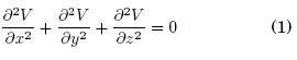
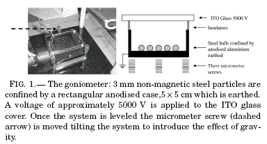
<body><![CDATA[<p align="justify">&nbsp;</p>     <p align="justify">&nbsp;</p>     <p align="justify"><font face="Verdana, Arial, Helvetica, sans-serif" size="3"><b>1.  INTRODUCCTION</b></font></p>     <p align="justify"><font face="Verdana, Arial, Helvetica, sans-serif" size="2">The physics of few-particle mesoscopic systems is an active and growing field of research. The scale of these systems is small enough for quantum effects to be considered, and yet of sufficient scale that classi-cal macroscopic laws still govern their behavior. Both experimental and theoretical approaches appear to support the assumption of an interparticle Coulomb interaction from which relatively simple macroscopic models emerge for several different systems, from nanotechnology to plasma research (Bonitz et al. 2008). However, crucial to research in this field is the determination and validation of the Coulomb interaction encouraging the development of new and in-teresting experiments at the macroscopic level and improving our understanding of phase transitions, packing of charged particles and other phenomena (Blonder 1985; Zheng &amp; Grieve 2006). While at the mesoscopic level, light is being shed on the role</font> <font face="Verdana, Arial, Helvetica, sans-serif" size="2">of quantum effects in the critical behavior of the Coulomb system (Clark et al. 2009).</font></p>     <p align="justify"><font face="Verdana, Arial, Helvetica, sans-serif" size="2">Over the years a number of theoretical models have been proposed with different repelling interac-tions, which include for example Coulomb, screened Coulomb, Lennard-Jones, dipole, logarithmic and hard sphere potentials (Jean et al. 2001; Schweigert et al. 1999). A recent experiment aimed at the determination and validation of the Coulomb interaction is that reported by (Zheng &amp; Grieve (2006); Ghezzi et al. (2008)) (and references therein) consisting of several millimeter-sized metallic spheres lying on the lower plate of a parallel plate square capacitor. The spheres are laterally confined by a square metallic electrically charged boundary which prevents their dispersion in 2 D. One of the con-clusions reached is that no dipole interaction is ob-served and hence the remaining reasonable option is the Coulomb interaction. Furthermore the deforma</font><font face="Verdana, Arial, Helvetica, sans-serif" size="2">tion of the ensemble of balls1 due to a gravitational gradient is measured inferring the nature of the re-pelling interaction aided by a computational method. This experiment belongs to a class of systems that are governed by the same physics, i.e., an interparticle interaction, a confining potential and an external potential (not to mention an eventual thermal activation). In the case that all of the above interactions have potentials that obey the Laplace equation with specific boundary conditions, we could then aim at numerically solving the equation of motion for the confined particles by means of the relaxation method where the physical interactions are incorporated via the corresponding boundary conditions in the confining border. In this work we take the experimental array referred to above (Zheng &amp; Grieve 2006; Ghezzi et al. 2008) and apply the Laplace equation to construct a minimal model. We understand by a &quot;minimal model&quot; one which contains just the sufficient number of essential features that would characterize the relevant physical phenomena in the system. In our case these features are: the Coulombian repulsion field among the particles (millimeter-sized metallic spheres), the confining field between the square metallic border and the particles, and the gravitational field acting upon the system when this is tilted at a certain angle.</font></p>     <p align="center"><a name="F1"></a><img src="/img/revistas/rbf/v33n33/a03_figura01.gif" width="384" height="207"></p>     <p align="justify">&nbsp;</p>     <p align="justify"><font face="Verdana, Arial, Helvetica, sans-serif" size="3"><b>2.  THE MODEL</b></font></p>     <p align="justify"><font face="Verdana, Arial, Helvetica, sans-serif" size="2">The model which corresponds to the square parallel plate capacitor (<a href="#F1">figure 1</a>) is a rectangular parallelepiped divided into 10 horizontal layers each containing 20 x 20 identical square boxes. When the tilting angle is zero the layers are perpendicular to the gravitational force, i.e., the system is level. The bottom and upper layers correspond to each of the parallel plates of the capacitor which have a definite electrical potential. The second layer from the bottom corresponds to the substrate in which the array of particles is located; only within this layer do the particles move according to the forces that yield the array to an equilibrium condition.</font></p>     <p align="justify"><font face="Verdana, Arial, Helvetica, sans-serif" size="2">By assigning a definite electrical potential value to the box occupied by any particle at a certain instant, we can reproduce the physical condition that all particles are equally charged; since the particles move, the box with this definite potential will also move while its neighboring boxes have a potential that is to be determined numerically by solving the Laplace equation</font> </p>     ]]></body>
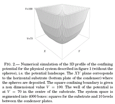
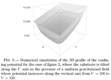
<body><![CDATA[<p align="center"><a name="E1"></a><img src="/img/revistas/rbf/v33n33/a03_figura02.gif" width="270" height="55"></p>     <p align="justify"><font face="Verdana, Arial, Helvetica, sans-serif" size="2">in a 3D lattice. For our purposes, one of the most important properties of the solution of (<a href="#E1">1</a>) is that the potential <i>V(x, y, z) </i>at some point (or box) is equal to the arithmetic mean of its six nearest neighbors in 3D,</font></p>     <p align="center"><a name="E2"></a><img src="/img/revistas/rbf/v33n33/a03_figura03.gif" width="366" height="55"></p>     <p align="justify"><font face="Verdana, Arial, Helvetica, sans-serif" size="2">where<i> <img src="/img/revistas/rbf/v33n33/a03_figura04.gif" width="172" height="19"></i>and similarly for <i><font face="Times New Roman, Times, serif">y</font> </i>and <i><font face="Times New Roman, Times, serif">z</font>. </i>The iterative numerical procedure by which (<a href="#E2">2</a>) converges to a definite value of the potential at every point of the lattice is the well known relaxation method [17]. For simplicity we will take here-after adimensional units for the potential <i><font face="Times New Roman, Times, serif">V(x, y, z)</font> </i>and for the coordinates <i><font face="Times New Roman, Times, serif">x, y, z</font> </i>with unit increments <i><font face="Arial, Helvetica, sans-serif">&Delta;x = &Delta;y = &Delta;z </font></i><font face="Arial, Helvetica, sans-serif">=</font> 1 in a square lattice.</font></p>     <p align="justify">&nbsp;</p>     <p align="justify"><font face="Verdana, Arial, Helvetica, sans-serif" size="3"><b>3.  ELECTRICAL PLUS GRAVITATIONAL POTENTIAL LANDSCAPES</b></font></p>     <p align="justify"><font face="Verdana, Arial, Helvetica, sans-serif" size="2">In order to avoid the dispersion of the particles due to the Coulombian repulsion, the square boundary has a definite potential which could be different from that of the particles but which we have considered as having the same potential in this work. This potential will be referred to as the &quot;confining potential&quot;. Thus, we construct a model where each particle is found in a &quot;potential landscape&quot; created by the parallel plates and the square boundary. Such potential landscape is calculated by implementing recursively (<a href="#E2">2</a>) through the whole parallelepiped divided in a grid of <font face="Times New Roman, Times, serif">10 x 20 x 20</font> boxes, although the relevant physics occurs in 2 D, that is, in the substrate where the particles would be allowed to move (<a href="#F2">figure 2</a>). Therefore, the potential landscape results from evaluating <i><font face="Times New Roman, Times, serif">V(x, y, z)</font> </i>vs. <font face="Times New Roman, Times, serif">(x, <i>y)</i></font><i> </i>keeping <i><font face="Times New Roman, Times, serif">z </font></i><font face="Times New Roman, Times, serif">= 2</font> constant (i.e., second layer from bottom to top). In <a href="#F2">figure 2</a> we have arbitrarily chosen the following boundary (non dimensional) values for the confining potential: <i><font face="Times New Roman, Times, serif">V(x, y, </font></i><font face="Times New Roman, Times, serif">1) = 99</font> for the bottom layer, <i><font face="Times New Roman, Times, serif">V(x, y, </font></i><font face="Times New Roman, Times, serif">10) = 0</font> for the top layer, <font face="Times New Roman, Times, serif">V(&plusmn;10, &plusmn;10, <i>z) </i>= 99</font> for the square boundary in each layer <font face="Times New Roman, Times, serif">(2 &lt; <i>z </i>&lt; 9)</font>. The origin of the <i><font face="Times New Roman, Times, serif">XY</font> </i>coordinate system of the layer where the particles are located is its geometrical center. In this landscape a single particle will move to the position with the minimum potential value, i.e., to the center of symmetry. When identical particles are included in the landscape, they will repel each other until all forces counterbalance and an equilibrium configuration is reached. Such a configuration is not so trivial to anticipate and a numerical evaluation of (<a href="#E2">2</a>) through the relaxation method is necessary even for a system with few particles.</font></p>     <p align="justify"><font face="Verdana, Arial, Helvetica, sans-serif" size="2">In <a href="#F3">figure 3</a> the potential landscape corresponds to a tilted substrate. In this case, the gravitational force manifests itself by means of a corresponding potential which increases uniformly in the positive <i><font face="Times New Roman, Times, serif">Y</font> </i>direction, i.e., <font face="Times New Roman, Times, serif">V(&plusmn;10, <i>y, </i>2) = <i>y </i>+ 109</font> . Interestingly, this gravitational potential is considered only as an</font> </p>     <p align="center"><a name="F2"></a><img src="/img/revistas/rbf/v33n33/a03_figura05.gif" width="382" height="345"></p>     <p align="center"><a name="F3"></a><img src="/img/revistas/rbf/v33n33/a03_figura06.gif" width="377" height="274"></p>     ]]></body>
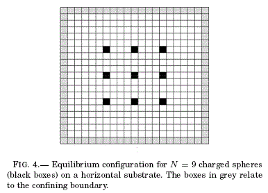
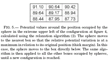
<body><![CDATA[<p align="justify"><font face="Verdana, Arial, Helvetica, sans-serif" size="2">additional boundary condition for the Laplace equation (<a href="#E1">1</a>) which is added to the existing electrical potential due to both the confining boundary and to the charged particles. Furthermore, the particles will move in the resulting potential landscape calculated using (<a href="#E2">2</a>) that contains <i><font face="Times New Roman, Times, serif">simultaneously</font> </i>both the electric and gravitational interactions. As can be seen in <a href="#F3">figure 3</a>, the particles will tend to move towards a different bottom position in this new potential landscape while repelling each other. This means that when compared to the level case, a different configuration of the particles will be reached.</font></p>     <p align="justify">&nbsp;</p>     <p align="justify"><font face="Verdana, Arial, Helvetica, sans-serif" size="3"><b>4.  DYNAMICS OF PARTICLES</b></font></p>     <p align="justify"><font face="Verdana, Arial, Helvetica, sans-serif" size="2">We chose the array of particles shown in <a href="#F4">figure 4</a> which is the equilibrium configuration when the substrate is level. In this symmetrical configuration of nine particles each particle produces a constant potential <i><font face="Times New Roman, Times, serif">V<sub>0</sub> = </font></i><font face="Times New Roman, Times, serif">99</font> in the box that it occupies. This potential <font face="Times New Roman, Times, serif"><i>V<sub>0</sub> = 99</i></font> is also a boundary condition for the Laplace equation when solved numerically by (<a href="#E2">2</a>). If this substrate is tilted the configuration in <a href="#F4">figure 4</a> is no longer in equilibrium and the particles will reach another final equilibrium configuration, i.e., each particle in <a href="#F4">figure 4</a> will start moving according</font> <font face="Verdana, Arial, Helvetica, sans-serif" size="2">to a dynamical rule that will be described below.</font></p>     <p align="center"><a name="F4"></a><img src="/img/revistas/rbf/v33n33/a03_figura07.gif" width="386" height="278"></p>     <p align="center"><a name="F5"></a><img src="/img/revistas/rbf/v33n33/a03_figura08.gif" width="376" height="212"></p>     <p align="justify"><font face="Verdana, Arial, Helvetica, sans-serif" size="2">Take for example the particle located at the point <font face="Times New Roman, Times, serif">(-4, 4)</font>, i.e., the particle at the upper left corner of the array in figure 4. Since this particle is considered as a &quot;test charge&quot;, its dynamical state can not be affected by its own potential but rather by the rest of the charges in the space. We therefore substitute the value of <font face="Times New Roman, Times, serif">V<sub>0</sub></font> at <font face="Times New Roman, Times, serif">(-4, 4)</font> by the algorithm (<a href="#E2">2</a>) and wait until the iterative routine stops. Then, we look at the potential values at <font face="Times New Roman, Times, serif">(-4, 4)</font> and its neighborhood. The result is shown in <a href="#F5">figure 5</a> where the heavy line border indicates the point <font face="Times New Roman, Times, serif">(-4,4)</font>.</font></p>     <p align="justify"><font face="Verdana, Arial, Helvetica, sans-serif" size="2">We notice by simple inspection that the potential at the point <font face="Times New Roman, Times, serif">(-4, 3)</font>, just below the position of the particle, is the least of the potential values of its four nearest boxes. Consequently, the particle will move to this new position and its corresponding box will be assigned the potential value V0 because the new test charge will be in another position, say at <font face="Times New Roman, Times, serif">(0,4)</font>. The process is repeated for the nine particles; the new resulting configuration will most probably be different from the original one.</font></p>     <p align="justify"><font face="Verdana, Arial, Helvetica, sans-serif" size="2">How can we be sure that these dynamics make physical sense? The total energy of the new configuration has to be less than that of the preceding configuration. When the particles in a configuration have nowhere else to move (because they are localized in the bottom of a local potential valley found around each particle) and the energy of such a configuration is at a minimum, we can assume that we have reached the final equilibrium configuration. However, realizing that such an energy is</font> <font face="Verdana, Arial, Helvetica, sans-serif" size="2">actually the minimum might not be an easy task, since it may correspond to a <i><font face="Times New Roman, Times, serif">metastable</font> </i>configuration which has less energy than its &quot;neighbor&quot; (or alike) configurations but has more energy than the real <i><font face="Times New Roman, Times, serif">stable</font> </i>equilibrium configuration. We can test, with some degree of reliability, if a configuration is stable or metastable by &quot;kicking&quot; the configuration, i.e., moving the particles to a neighboring position, not necessarily the nearest, and comparing the energy changes. If the energy always grows after a few kicks, the configuration is most probably stable; if the energy diminishes after a few kicks, the configuration is metastable. Of course it is not guaranteed that the new configuration will be a stable one, because there could exist many metastable configurations, and the kicks may simply take the system from one configuration to another.</font></p>     <p align="justify"><font face="Verdana, Arial, Helvetica, sans-serif" size="2">Another word of caution: the dynamical process leading to a final equilibrium configuration, although it might have physical sense, need not be the <i><font face="Times New Roman, Times, serif">real</font> </i>dynamical process observed in an actual experiment. This is because in our model the allowed displacement of the particles is one box, either in the <i><font face="Times New Roman, Times, serif">X</font> </i>or <i><font face="Times New Roman, Times, serif">Y</font> </i>direction, per configuration. In a real experiment, each new configuration is defined by the instant positions of the particles, i.e., if <i><font face="Times New Roman, Times, serif">T</font> </i>is the total time elapsed from the initial to the final configurations and we want to have <i><font face="Times New Roman, Times, serif">N</font> </i>configurations, then one particular configuration corresponds to the positions of the particles at the time <i><font face="Times New Roman, Times, serif">t = nT/N</font>, </i>with the integer <font face="Times New Roman, Times, serif">n</font> in the interval <font face="Times New Roman, Times, serif">0 &lt; <i>n &lt; N</i></font><i>. </i>Therefore, in a real experiment, the particles' displacements could all be different, both in magnitude and direction. Nevertheless, and being conscious that the modeled dynamics can be different from the real one, we claim that the final equilibrium configuration characterized by a unique minimum of the total energy, <i><font face="Times New Roman, Times, serif">isthesameinanycase</font>. </i>Differences will arise depending on how gross is the lattice's grid segmentation of the lattice's, i.e., the size of the box, which in turn will cause the equilibrium configuration to be reached in a longer time than the real one. Another possible difference is that in the model dynamics, a coarse grid segmentation will yield a final stationary oscillating state in which two different configurations (with a negligible energy difference) alternate, such that the real final configuration, having the minimum energy, can never be reached. The claim mentioned above is the matter of our current research and lies beyond the scope of this work.</font></p>     ]]></body>
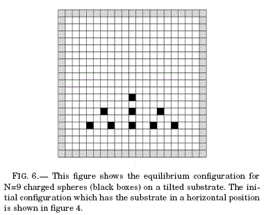
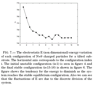
<body><![CDATA[<p align="justify"><font face="Verdana, Arial, Helvetica, sans-serif" size="2">In <a href="#F6">figure 6</a> we have the final equilibrium configuration corresponding to the initial state depicted in <a href="#F4">figure 4</a> (in both cases we observe only the layer where the particles move). The black boxes represent the positions of the particles and the grey boxes determine the square confining boundary. The corresponding energy evolution is depicted in <a href="#F7">figure 7</a> (with energy values in the vertical axis and configuration index in the horizontal axis) where there are 13 different configurations including the initial and the final ones. The difference among configurations is not deduced from their energies; it was observed while</font> <font face="Verdana, Arial, Helvetica, sans-serif" size="2">the model dynamics were in course. Notice one interesting thing: the eighth and tenth configurations have less energy than the -supposedly- final configuration (the thirteenth) but in those configurations the particles had other allowed positions to move to, so we preferred to continue the model dynamics until it stopped or until it reached a stationary oscillating state. The former occurred first.</font></p>     <p align="center"><a name="F6"></a><img src="/img/revistas/rbf/v33n33/a03_figura09.gif" width="383" height="309"></p>     <p align="center"><a name="F7"></a><img src="/img/revistas/rbf/v33n33/a03_figura10.gif" width="381" height="345"></p>     <p align="center">&nbsp;</p>     <p align="justify"><font face="Verdana, Arial, Helvetica, sans-serif" size="3"><b>5.  CONFINING AND REPULSIVE FORCE FIELDS</b></font></p>     <p align="justify"><font face="Verdana, Arial, Helvetica, sans-serif" size="2">Next, once we achieve the potential energy field corresponding to <a href="#F6">figure 6</a>, we can deduce its vector force field. This is done by implementing</font></p>     <p align="center"><a name="E3"></a><img src="/img/revistas/rbf/v33n33/a03_figura11.gif" width="284" height="49"></p>     <p align="justify"><font face="Verdana, Arial, Helvetica, sans-serif" size="2">for each particle in the 2D substrate lattice. We are purportedly ignoring the forces that are perpendicular to the substrate because they will cancel out with the corresponding normal forces. The derivative of <i><font face="Times New Roman, Times, serif">V(x, y)</font> </i>with respect to <i>x </i>is (recall that we have set</font> <font face="Times New Roman, Times, serif" size="2">&Delta;<i>x</i> = &Delta;<i>y</i> = &Delta;<i>z</i>= 1</font><font face="Verdana, Arial, Helvetica, sans-serif" size="2"> in this work)</font></p>     <p align="center"><a name="F8"></a><img src="/img/revistas/rbf/v33n33/a03_figura12.gif" width="403" height="344"></p>     <p align="center"><a name="E4"></a><img src="/img/revistas/rbf/v33n33/a03_figura13.gif" width="269" height="42"></p>     ]]></body>
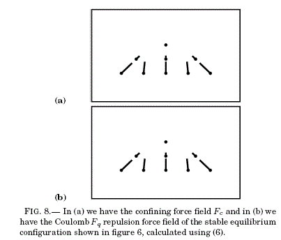
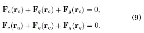
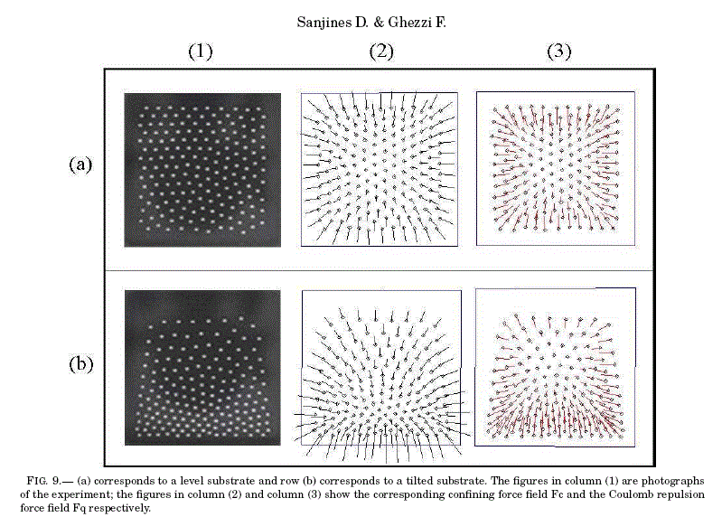
<body><![CDATA[<p align="justify"><font face="Verdana, Arial, Helvetica, sans-serif" size="2">from which one can write</font></p>     <p align="center"><a name="E5"></a><img src="/img/revistas/rbf/v33n33/a03_figura14.gif" width="307" height="40"></p>     <p align="justify"><font face="Verdana, Arial, Helvetica, sans-serif" size="2">thus (<a href="#E3"><b>3</b></a>) results in</font></p>     <p align="center"><a name="E6"></a><img src="/img/revistas/rbf/v33n33/a03_figura15.gif" width="318" height="42"></p>     <p align="justify"><font face="Verdana, Arial, Helvetica, sans-serif" size="2">The confining force field in <a href="#F8">figure 8a</a> was obtained by applying (<a href="#E6">6</a>) to each of the equilibrium positions in <a href="#F6">figure 6</a> once the gravitational potential was set to zero (level substrate) and the <i><font face="Times New Roman, Times, serif">V<sub>0</sub></font> </i>potential of each charge was substituted by the relaxation algorithm (<a href="#E2">2</a>). Therefore, the resulting potential landscape </font><font size="2" face="Times New Roman, Times, serif"><i>V<sub>c </sub></i></font><font face="Verdana, Arial, Helvetica, sans-serif" size="2">corresponds <i><font face="Times New Roman, Times, serif">only</font> </i>to the confining interaction due to the charged boundary (lateral, top and bottom plates). In a similar way, we have obtained the repulsive force field among particles (<a href="#F8">figure 8b</a>) by applying (<a href="#E6">6</a>) to the potential field <i><font face="Times New Roman, Times, serif">V<sub>cq</sub>?V<sub>c</sub></font> </i>resulting in the subtraction of the confining potential field <i>(<font face="Times New Roman, Times, serif">V<sub>c</sub></font>) </i>from the potential field due to both the confining and Coulomb interactions among particles <i>(<font face="Times New Roman, Times, serif">V<sub>cq</sub></font>).</i></font></p>     <p align="justify"><font face="Verdana, Arial, Helvetica, sans-serif" size="2">We now recall that the equilibrium condition tak-ing into account all the interactions is</font></p>     <p align="center"><a name="E7"></a><img src="/img/revistas/rbf/v33n33/a03_figura16.gif" width="298" height="33"></p>     <p align="justify"><font face="Verdana, Arial, Helvetica, sans-serif" size="2">where <font face="Times New Roman, Times, serif"><b>F</b><sub><i>c</i></sub>(<b>r</b><sub><i>i</i></sub>)</font> and <font face="Times New Roman, Times, serif"><b>F</b><sub>q</sub>(<b>r</b><sub><i>i</i></sub>)</font> are the vector fields corresponding to the confining and repulsive forces respectively (<a href="#F8">figure 8</a>) and <font face="Times New Roman, Times, serif">r<sub><i>i</i></sub></font> is the respective position of the nine particle array; <i><font face="Times New Roman, Times, serif">m<b>g</b>sen&Theta;</font> </i>is the field of &quot;residua&quot; forces corresponding to the gravitational interaction. Then, should the whole method applied in this work be consistent, it is expected that the gravitational force field can be obtained from the <font face="Times New Roman, Times, serif"><b>F</b><sub>c</sub></font> and <font face="Times New Roman, Times, serif"><b>F</b><sub>q</sub></font> fields according to (<a href="#E7">7</a>).</font></p>     <p align="justify"><font face="Verdana, Arial, Helvetica, sans-serif" size="2"><a href="#F9">Figure 9</a> shows the corresponding confining (a) and repulsive (b) force fields for an actual experiment</font> <font face="Verdana, Arial, Helvetica, sans-serif" size="2">with a system of 169 particles (<a href="#E16">16</a>). A distinctive feature that can be observed when one compares this latter figure with the simulated experiment in <a href="#F8">figure 8</a> is that in both cases there appears a kind of &quot;equilibrium center&quot; where the force is null, being the equilibrium center of the confining field in an upper position with respect to the center of the repulsive field. We can show that in the case of a level substrate these two equilibrium centers coincide; for a tilted substrate (as in <a href="#F9">figure 9</a>) the distance between equilibrium centers will be proportional to some monotonous function of the angle of inclination. Knowing the particles configuration in equilibrium, it follows that we can obtain the residual gravitational force value <font face="Times New Roman, Times, serif"><b>F</b><sub><i>g</i></sub></font> . To this end (<a href="#E7">7</a>) is written as</font></p>     <p align="center"><a name="E8"></a><img src="/img/revistas/rbf/v33n33/a03_figura17.gif" width="290" height="35"></p>     ]]></body>
<body><![CDATA[<p align="justify"><font face="Verdana, Arial, Helvetica, sans-serif" size="2">and the expression is applied to the centres of equilibrium of charge <font face="Times New Roman, Times, serif"><b>r</b><sub><i>q</i></sub></font> and confinement <font face="Times New Roman, Times, serif"><b>r</b><sub><i>q</i></sub></font> that are assumed to be known through the configuration of the particles:</font></p>     <p align="center"><a name="E9"></a><img src="/img/revistas/rbf/v33n33/a03_figura18.gif" width="295" height="69"></p>     <p align="justify"><font face="Verdana, Arial, Helvetica, sans-serif" size="2">According to the hypothesis <font face="Times New Roman, Times, serif"><b>F</b><sub><i>q</i></sub>(<b>r</b><i><sub>q</sub></i>) = <b>F</b><i><sub>c</sub></i>(<b>r</b><i><sub>c</sub></i>) = 0 <font face="Verdana, Arial, Helvetica, sans-serif">and</font> <b>F</b><i><sub>g</sub></i>(<b>r</b>) = <b>F</b><sub><i>g</i></sub> = <i>const. </i><font face="Verdana, Arial, Helvetica, sans-serif">(for any <b><font face="Times New Roman, Times, serif">r</font></b>)</font></font>, it follows <font face="Times New Roman, Times, serif"><b>F</b><i><sub>g</sub></i> = -<b>F</b><i><sub>q</sub></i>(<b>r</b><i><sub>c</sub></i>) = -<b>F</b><sub><i>c</i></sub>(<b>r</b><i><sub>q</sub></i>)</font>. In view of the symmetry of the confinement field F<sub>c</sub> as a consequence of the form (square) of the confinement border and the independent nature of the field in relation to the configuration of the particles in equilibrium, it is deemed better to evaluate the residual gravitational field in agreement with</font></p>     <p align="center"><a name="E10"></a><img src="/img/revistas/rbf/v33n33/a03_figura19.gif" width="243" height="28"></p>     <p align="justify"><font face="Verdana, Arial, Helvetica, sans-serif" size="2">Given that the confinement and gravitational fields are unique (for certain gradients of a tilted substrate) for the earlier expression (<a href="#E10">10</a>) it is suggested that the centre of equilibrium of charge <font face="Times New Roman, Times, serif"><b>r</b><i><sub>q</sub></i></font> is the same <i><font face="Times New Roman, Times, serif">irrespective of the number of particles</font>. </i>This speculation and also the efficient use of (<a href="#E10">10</a>) to calculate the residual gravitational force field are interesting areas for further investigation.</font></p>     <p align="justify">&nbsp;</p>     <p align="justify"><font face="Verdana, Arial, Helvetica, sans-serif" size="3"><b>6.  ERROR ESTIMATION</b></font></p>     <p align="justify"><font face="Verdana, Arial, Helvetica, sans-serif" size="2">A state of equilibrium (<a href="#E7">7</a>) is equivalent to having a minimum energy in each site containing a particle. However, given that the error estimation in the 2D lattice is due to the finite size of a cell, then (<a href="#E4">4</a>) shows a minimum energy potential error of <font face="Verdana, Arial, Helvetica, sans-serif" size="2"><font face="Times New Roman, Times, serif">&Delta;</font><i><font face="Times New Roman, Times, serif">V<sub>x</sub>+ - V = V - V<sub>x</sub>-</font> </i></font> along the <i>X </i>axis and an error of <font face="Times New Roman, Times, serif">&Delta;<i>V<sub>y</sub> </i>=</font> <i><font face="Times New Roman, Times, serif">V<sub>y</sub>+ - V = V - V<sub>y</sub>-</font> </i>along the <i>Y </i>axis. The corresponding errors in the force components acting on each particle are</font></p>     <p align="center"><a name="E11"></a><img src="/img/revistas/rbf/v33n33/a03_figura20.gif" width="335" height="65"></p>     <p align="center"><a name="F9"></a><img src="/img/revistas/rbf/v33n33/a03_figura21.gif" width="799" height="572"></p>     ]]></body>
<body><![CDATA[<p align="justify"><font face="Verdana, Arial, Helvetica, sans-serif" size="2">this would lead to the rewriting of (<a href="#E6">6</a>) to include the follo wing error:</font></p>     <p align="center"><a name="E12"></a><img src="/img/revistas/rbf/v33n33/a03_figura22.gif" width="366" height="28"></p>     <p align="justify"><font face="Verdana, Arial, Helvetica, sans-serif" size="2"><i><font face="Times New Roman, Times, serif">F</font> </i>is the net force on each particle, where <b><font face="Times New Roman, Times, serif">F</font></b>&deg; is the computed force and its corresponding error <font face="Times New Roman, Times, serif">&Delta;<b>F</b></font> is due to the cell dimensions. Now we demonstrate that <font face="Times New Roman, Times, serif">|&Delta;<i>F<sub>x</sub></i>| =<i> |</i>&Delta;<i>F<sub>y</sub></i>|</font> in (<a href="#E12">12</a>). Taking into account that the particles only move within the <i><font face="Times New Roman, Times, serif">XY</font> </i>plane of the substrate, there should not exist a net force along the <i><font face="Times New Roman, Times, serif">Z</font> </i>axis perpendicular to the substrate. This translates into the condition <i><font face="Times New Roman, Times, serif">V<sub>z</sub>+ = V<sub>z</sub>-<sub>=V</sub></font> </i>in expression (2), where we obtain</font></p>     <p align="center"><a name="E13"></a><img src="/img/revistas/rbf/v33n33/a03_figura23.gif" width="343" height="42"></p>     <p align="justify"><font face="Verdana, Arial, Helvetica, sans-serif" size="2">Substituting this in (<a href="#E11">11</a>) instead of V and readjusting terms we obtain the desired result</font></p>     <p align="center"><a name="E14"></a><img src="/img/revistas/rbf/v33n33/a03_figura24.gif" width="371" height="39"></p>     <p align="justify"><font face="Verdana, Arial, Helvetica, sans-serif" size="2">If we consider <font face="Times New Roman, Times, serif"><b>F</b>&deg; = F&deg;<b>f</b></font>, defining <i><font face="Times New Roman, Times, serif">&alpha; =</font> </i><font face="Times New Roman, Times, serif">|&Delta;<i>F<sub>x</sub></i>| =<i> |</i>&Delta;<i>F<sub>y</sub></i>|</font> from (<a href="#E14">14</a>), then the error of <font face="Times New Roman, Times, serif"><b>F</b>&deg;</font> in (<a href="#E12">12</a>) should be</font></p>     <p align="center"><a name="E15"></a><img src="/img/revistas/rbf/v33n33/a03_figura25.gif" width="259" height="30"></p>     <p align="justify"><font face="Verdana, Arial, Helvetica, sans-serif" size="2">where &fnof; is unitary in the direction of <font face="Times New Roman, Times, serif"><b>F</b>&deg;</font> . It can be seen in (<a href="#E15">15</a>) that the error <font face="Times New Roman, Times, serif">&Delta;<b>F</b></font> affects as much the magnitude as it does the direction of <font face="Times New Roman, Times, serif"><b>F</b>&deg;</font> . We can reasonably assume that both magnitude and directional</font> <font face="Verdana, Arial, Helvetica, sans-serif" size="2">errors are of the order<i><font face="Times New Roman, Times, serif"> &alpha; </font></i>and as such (<a href="#E12">12</a>) is written as</font></p>     <p align="center"><a name="E16"></a><img src="/img/revistas/rbf/v33n33/a03_figura26.gif" width="266" height="32"></p>     ]]></body>
<body><![CDATA[<p align="justify"><font face="Verdana, Arial, Helvetica, sans-serif" size="2">where <font size="3" face="Times New Roman, Times, serif">|&xi;| &lt; <i>&alpha;</i></font><font size="3"> <font size="2">and</font> <i><font face="Times New Roman, Times, serif"> |&eta;|&lt;</font><font face="Verdana, Arial, Helvetica, sans-serif" size="2"><font size="3" face="Times New Roman, Times, serif"><i>&alpha;</i></font></font></i></font> (note that <i><font size="3" face="Times New Roman, Times, serif">&alpha;,&xi;</font></i> and <i><font size="3" face="Times New Roman, Times, serif">&eta;</font> </i>have units of force). Developing (<a href="#E16">16</a>) we arrive at the expression</font></p>      <p align="center"><a name="E17"></a><img src="/img/revistas/rbf/v33n33/a03_figura27.gif" width="371" height="39"></p>     <p align="justify"><font face="Verdana, Arial, Helvetica, sans-serif" size="2">where <i><font face="Times New Roman, Times, serif">F</font> </i>is the magnitude of <font face="Times New Roman, Times, serif"><b>F</b>&deg;</font> and <i><font face="Times New Roman, Times, serif">F<sub>x</sub>, F<sub>y</sub></font> </i>are its respective components. When necessary hereafter we will distinguish the magnitude and components of <b><font face="Times New Roman, Times, serif">F</font></b> from those of <b><font face="Times New Roman, Times, serif">F</font></b><font face="Times New Roman, Times, serif">&deg;</font> by adding the superscript for this last case.</font></p>     <p align="justify"><font face="Verdana, Arial, Helvetica, sans-serif" size="2">When <font size="3" face="Times New Roman, Times, serif"><i>&xi;</i></font> y <font size="3" face="Times New Roman, Times, serif"><i>&eta;</i></font> are simultaneously zero in (<a href="#E17">17</a>), then <font face="Times New Roman, Times, serif"><b>F</b> = <b>F</b>&deg;</font>, as expected. However, we know that for physical reasons if <b><font face="Times New Roman, Times, serif">F</font></b> represents the residual force field corresponding to the gravity component along the inclined substrate in the direction of axis <i><font face="Times New Roman, Times, serif">Y</font> </i>(<a href="#F3">figure 3</a>), then from (<a href="#E7">7</a>) we have that the sum of the confining force <font face="Times New Roman, Times, serif"><b>F</b><sub>c</sub></font> and the Coulombian repulsion <b><font face="Times New Roman, Times, serif"><i>F</i></font></b><font face="Times New Roman, Times, serif"><i><sub>q</sub></i></font> should only contain components along the <i><font face="Times New Roman, Times, serif">Y</font> </i>axis. As such, the <b><font face="Times New Roman, Times, serif">F</font></b> components along the <i><font face="Times New Roman, Times, serif">X</font> </i>axis in (17) should be null for all particles. As we can see in graphs (a) and (b) of <a href="#F8">figure 8</a>, <font face="Times New Roman, Times, serif"><b>F</b><sub>c</sub> + <b><i>F</i></b><i><sub>q</sub></i></font> do not have null components along the <i><font face="Times New Roman, Times, serif">X</font> </i>axis, we suppose that this is due to the errors discussed. Hence, equation (<a href="#E17">17</a>) is subject to the following restriction</font></p>     <p align="center"><a name="E18"></a><img src="/img/revistas/rbf/v33n33/a03_figura28.gif" width="278" height="27"></p>     <p align="justify"><font face="Verdana, Arial, Helvetica, sans-serif" size="2">which results in <font face="Times New Roman, Times, serif"><i>F</i></font><i> </i>components only along the <i><font face="Times New Roman, Times, serif">Y</font> </i>axis in (<a href="#E17">17</a>). Substituting the value <i><font size="3" face="Times New Roman, Times, serif">&eta;</font></i> of (<a href="#E18">18</a>) in (<a href="#E17">17</a>) we obtain</font></p>     <p align="center"><a name="E19"></a><img src="/img/revistas/rbf/v33n33/a03_figura29.gif" width="253" height="27"></p>     <p align="justify"><font face="Verdana, Arial, Helvetica, sans-serif" size="2">or equivalently</font></p>     <p align="center"><a name="E20"></a><img src="/img/revistas/rbf/v33n33/a03_figura30.gif" width="357" height="39"></p>     <p align="justify"><font face="Verdana, Arial, Helvetica, sans-serif" size="2">where the subscript <font size="3" face="Times New Roman, Times, serif"><i>i</i></font><font size="3"> </font>represents each one of the particles. So the <font face="Times New Roman, Times, serif"><i>F</i></font> field in (<a href="#E19">19</a>) is seen as a set of aligned vectors along the <font face="Times New Roman, Times, serif"><i>Y</i></font> axis with different magnitudes. According to (<a href="#E7">7</a>) these magnitudes should be equal. For this to happen we should apply the appropriate values of <font size="3" face="Times New Roman, Times, serif"><i>&xi;<sub>i</sub></i></font> for each particle. This is a time consuming and cumbersome process and we have therefore chosen the following criteria. We consider a unique value of <font size="3" face="Times New Roman, Times, serif">&xi;</font> in (<a href="#E20">20</a>) for all the particles and define the deviation as <font face="Times New Roman, Times, serif"><i><font size="3">d<sub>i</sub></font></i><font size="3"> = <i>F<sub>y,i</sub> - F&deg;<sub>y,i</sub></i></font> <font face="Verdana, Arial, Helvetica, sans-serif">so that</font> <font size="3"><i>S(&xi;)</i></font> = <font size="3">&sum;<sub><i>i</i></sub><i> d</i><sup>2</sup><sub><i>i</i></sub></font></font> has a minimum value, i.e., <font size="3" face="Times New Roman, Times, serif"><i>&eth;</i><sub><i>&xi;</i></sub> <i>S</i></font><font face="Times New Roman, Times, serif"> = </font><font face="Times New Roman, Times, serif">0</font> and we obtain</font></p>     ]]></body>
<body><![CDATA[<p align="center"><a name="E21"></a><img src="/img/revistas/rbf/v33n33/a03_figura31.gif" width="272" height="53"></p>     <p align="justify"><font face="Verdana, Arial, Helvetica, sans-serif" size="2">where <font size="3" face="Times New Roman, Times, serif">&xi;</font> only guarantees a minimum value of <font face="Times New Roman, Times, serif"><i>F</i><sub>y,i</sub></font> in (<a href="#E20">20</a>) with respect to an average value of<i><font face="Times New Roman, Times, serif"> F<sub><i>y,i</i></sub></font></i>over all the particles <i><font face="Times New Roman, Times, serif">N</font> </i>defined as</font></p>     <p align="center"><a name="E21"></a><img src="/img/revistas/rbf/v33n33/a03_figura32.gif" width="372" height="51"></p>     <p align="justify"><font face="Verdana, Arial, Helvetica, sans-serif" size="2">This expression provides a useful numerical estimation of the residual gravitational force that is obtained in the experimental set up when the plane is inclined. Thus, there must be a linear relationship between <i><font face="Times New Roman, Times, serif">(F<sub>y</sub></font></i><font face="Times New Roman, Times, serif">)</font> the values and sine of the inclination angle.</font></p>     <p align="justify"><font face="Verdana, Arial, Helvetica, sans-serif" size="2">Note that when a substrate is horizontal it is likely that some or all of the <i><font size="3" face="Times New Roman, Times, serif">F&deg;<sub>y,i</sub></font></i> values will be zero. In these cases (<a href="#E18">18</a>) is used instead of (<a href="#E22">22</a>) where <font size="3" face="Times New Roman, Times, serif">&xi; = <i>-F<sub>x</sub> = -F</i></font> is obtained. In this case we need to define <font size="3" face="Times New Roman, Times, serif"><b>F</b> = 0j</font> to avoid an undetermined result in (<a href="#E19">19</a>).</font></p>     <p align="justify"><font face="Verdana, Arial, Helvetica, sans-serif" size="2">We apply (<a href="#E22">22</a>) for a substrate at 4 different gradients such that <i><font face="Times New Roman, Times, serif">&theta;<sub>1</sub> &gt; &theta;<sub>2</sub> &gt; &theta;<sub>3</sub> &gt; &theta;<sub>4</sub> </font></i><font face="Times New Roman, Times, serif">&gt;</font>. Since the gravitational field is homogeneous, the energy potential variation along the <font face="Times New Roman, Times, serif">Z</font> axis (<a href="#F3">figure 3</a>) is <font size="3" face="Times New Roman, Times, serif">&Delta;<i>V</i> = <i>mgAz</i></font><i>, </i>where m is the mass of each particle. So, the substrate slope is <font size="3" face="Times New Roman, Times, serif">&Delta;z/&Delta;x = <i>tan</i> = &Delta;<i>V</i>/(mg&Delta;x)</font><i>. </i>Since in this study the value of <font face="Times New Roman, Times, serif">&Delta;<i>V</i></font> is not given in physical units but is non dimensional, and the mass of the spheres is an unknown parameter, we can only compare the different gradients among them and draw conclusions. The <i>9 </i>angles are unknown but their ratios are known. The selected values are</font></p>     <p align="center"><a name="E23"></a><img src="/img/revistas/rbf/v33n33/a03_figura33.gif" width="318" height="32"></p>     <p align="justify"><font face="Verdana, Arial, Helvetica, sans-serif" size="2">where the configuration of <a href="#F6">figure 6</a> corresponds to <font size="3" face="Times New Roman, Times, serif"><i>&theta;</i><sub>3</sub></font>. For the configurations corresponding to the gradients given in (<a href="#E23">23</a>), the non dimensional residual force values <font size="3" face="Times New Roman, Times, serif"><i>F<sub>i</sub></i> <i>(F<sub>y</sub> </i>=)</font> shown in (<a href="#E22">22</a>) are <i><font size="3" face="Times New Roman, Times, serif">F<sub>i</sub> = 1.360, F<sub>2</sub> = 0.839, F<sub>3</sub> = 0.725, F<sub>4</sub> = 0.225</font></i>, and from which</font> <font face="Verdana, Arial, Helvetica, sans-serif" size="2">the relevant quotients <i><font size="3" face="Times New Roman, Times, serif">F<sub>i,j</sub> = F<sub>i</sub>/F<sub>j</sub></font> </i>are constructed:</font></p>     <p align="center"><a name="E24"></a><img src="/img/revistas/rbf/v33n33/a03_figura34.gif" width="333" height="47"></p>     <p align="justify"><font face="Verdana, Arial, Helvetica, sans-serif" size="2">Additionally, defining <font size="3"><font face="Times New Roman, Times, serif"><i>&xi;<sub>i,j</sub> = (sen&theta;i/sen&theta;j)<sup>2</sup></i></font></font> , the relations in (<a href="#E23">23</a>) are expressed as</font></p>     ]]></body>
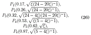
<body><![CDATA[<p align="center"><a name="E25"></a><img src="/img/revistas/rbf/v33n33/a03_figura35.gif" width="297" height="33"></p>     <p align="justify"><font face="Verdana, Arial, Helvetica, sans-serif" size="2">and combine together with <i><font size="3" face="Times New Roman, Times, serif">&xi;<sub>i,j</sub>&xi;<sub>j,k</sub> = &xi;<sub>i,k</sub></font></i> and <font size="3" face="Times New Roman, Times, serif"><i>&xi;<sub>i,j</sub> = &xi;<sup>-1</sup><sub>j,i</sub></i></font> (according to the definition of <font size="3" face="Times New Roman, Times, serif"><i>&xi;<sub>i,j</sub></i></font>) to obtain all of</font> <font face="Verdana, Arial, Helvetica, sans-serif" size="2">the relevant combinations: <i><font size="3" face="Times New Roman, Times, serif">&xi;<sub>4,3</sub>, &xi;<sub>4,2</sub>, &xi;<sub>4,1</sub> , &xi;<sub>3,2</sub> , &xi; <sub>3,1</sub>, &xi;<sub>2,1</sub></font></i>. These values together with those of (<a href="#E24">24</a>) serve to construct the points <font face="Verdana, Arial, Helvetica, sans-serif" size="2"><font face="Times New Roman, Times, serif"><img src="/img/revistas/rbf/v33n33/a03_figura39.gif" width="94" height="19"></font></font><font face="Times New Roman, Times, serif">, </font>These are used to verify if <font size="3"><i><font face="Times New Roman, Times, serif">F<sub>i</sub> &alpha; sen &theta;<sub>i</sub></font></i></font><i> , </i>where the gradient <i><font size="3" face="Times New Roman, Times, serif">m</font></i> of a linear adjustment of the points <i><font size="3" face="Times New Roman, Times, serif">P</font> </i>should be close to 1. These points, ordered in ascending value of the abscissa, are</font></p>     <p align="center"><a name="E226"></a><img src="/img/revistas/rbf/v33n33/a03_figura36.gif" width="311" height="122"></p>     <p align="justify"><font face="Verdana, Arial, Helvetica, sans-serif" size="2">We define <i><font size="3" face="Times New Roman, Times, serif">&xi; = &xi;<sub>2,1</sub></font></i> as a variable parameter of which the gradient <i><font size="3" face="Times New Roman, Times, serif">m(&xi;)</font></i> is dependent. The validity interval of <i><font size="3" face="Times New Roman, Times, serif">&xi;</font></i> is calculated from the first relation in (<a href="#E23">23</a>) obtaining:</font></p>     <p align="center"><a name="E27"></a><img src="/img/revistas/rbf/v33n33/a03_figura37.gif" width="275" height="44"></p>     <p align="justify"><font face="Verdana, Arial, Helvetica, sans-serif" size="2">Given that in (<a href="#E27">27</a>) the minimum value of <font size="3" face="Times New Roman, Times, serif"><i>&theta;<sub>2</sub></i></font> is <font size="3" face="Times New Roman, Times, serif"><i>&theta;&deg;</i></font> and the maximum value of <font size="3" face="Times New Roman, Times, serif"><i>&theta;<sub>2</sub></i></font> is <font size="3" face="Times New Roman, Times, serif">90&deg;</font>, we obtain <font face="Times New Roman, Times, serif">0.25 &lt; <i>&xi;</i> &lt; 1</font>, then the slope <i><font size="3" face="Times New Roman, Times, serif">m(&xi;)</font></i> for the 6 points in (<a href="#E26">26</a>) is calculated using a linear fitting leading to an ascending monotonous function with extreme values <i><font size="3" face="Times New Roman, Times, serif">m(</font></i><font size="3" face="Times New Roman, Times, serif">0.25<i>)</i></font><font face="Times New Roman, Times, serif"> <img src="/img/revistas/rbf/v33n33/a03_figura40.gif" width="11" height="12"> 0.46, <i><font size="3">m(</font></i><font size="3">1</font><i><font size="3">)</font> </i><font face="Verdana, Arial, Helvetica, sans-serif" size="2"><img src="/img/revistas/rbf/v33n33/a03_figura40.gif" width="11" height="12"></font> 0.9</font> and mean values <font size="3" face="Times New Roman, Times, serif">(<i>m</i>) = 0.67</font>. Since we have</font></p>     <p align="center"><a name="E28"></a><img src="/img/revistas/rbf/v33n33/a03_figura38.gif" width="242" height="47"></p>     <p align="justify"><font face="Verdana, Arial, Helvetica, sans-serif" size="2">then the numerical results for m indicate that the relation<font size="3"><i><font face="Times New Roman, Times, serif"> F<sub>i</sub> &alpha; sen &theta;<sub>i</sub></font></i></font> is reasonably satisfactory <font size="3" face="Times New Roman, Times, serif">(<i>m</i> </font><font face="Verdana, Arial, Helvetica, sans-serif" size="2"><font face="Times New Roman, Times, serif"><font face="Verdana, Arial, Helvetica, sans-serif" size="2"><img src="/img/revistas/rbf/v33n33/a03_figura40.gif" width="11" height="12"></font></font></font><font size="3" face="Times New Roman, Times, serif"> 0.93)</font> when the gradients are big <i>(<font size="3" face="Times New Roman, Times, serif">&theta;<sub>1</sub> </font></i><font size="3" face="Times New Roman, Times, serif"><img src="/img/revistas/rbf/v33n33/a03_figura40.gif" width="11" height="12"> 90&deg;</font>). The discrepancies resulting from smaller gradients are at-tributed in this work to the coarse segmentation of the substrate (20 x 20 boxes) and the small number of particles <i>(<font size="3" face="Times New Roman, Times, serif">N = </font></i><font size="3" face="Times New Roman, Times, serif">9</font>) involved which do no result in reliable residual force values in (<a href="#E22">22</a>).</font></p>     <p align="justify">&nbsp;</p>     <p align="justify"><font face="Verdana, Arial, Helvetica, sans-serif" size="3"><b>7.  CONCLUSIONS</b></font></p>     ]]></body>
<body><![CDATA[<p align="justify"><font face="Verdana, Arial, Helvetica, sans-serif" size="2">We have constructed a &quot;minimal&quot; model to reproduce relevant features of a system of several electri-cally charged particles confined in a square parallel plate capacitor. Our approach embraces the theory of <font face="Times New Roman, Times, serif"><i>r</i><sup>-2</sup></font> type interactions as well as data from actual experiments and numerical simulation.</font></p>     <p align="justify"><font face="Verdana, Arial, Helvetica, sans-serif" size="2">The method employed for such a purpose is the solution of the Laplace equation in 3D by means of the relaxation method. The main results in this work are: (i) the final equilibrium configuration of a</font> <font face="Verdana, Arial, Helvetica, sans-serif" size="2">system of 9 particles, (ii) the corresponding energy evolution through the intermediate non-equilibrium configurations, and (iii) the vector force fields for the confining and repulsive interactions. These results are compared with those of the actual experimental set up with many particles (e.g., <a href="#F9">figure 9</a> with 169 particles) and a qualitative good agreement is found.</font></p>     <p align="justify"><font face="Verdana, Arial, Helvetica, sans-serif" size="2">In this work, the solution of the Laplace equation is a scalar field of potential which can incorporate <i><font face="Times New Roman, Times, serif">simultaneously</font> </i>all the different physical interactions (e.g., electrical and gravitational) as boundary conditions for the solution of the Laplace equation. The resulting vector force field deduced from the total potential field thus determines the dynamical behavior of the particles and the stable equilibrium configuration of the system.</font></p>     <p align="justify"><font face="Verdana, Arial, Helvetica, sans-serif" size="2">Emerging from this work was the concept of an &quot;equilibrium center&quot; for the force fields (confining and repulsive) which may provide an alternative way for determining global characteristics of the particle system. Such an equilibrium center could move in an analogous way as does the center of mass of a particle system when acted upon by external forces.</font></p>     <p align="justify"><font face="Verdana, Arial, Helvetica, sans-serif" size="2">Furthermore, we modeled the dynamics of the particles using a specific algorithm which results in a final equilibrium configuration exhibiting a minimum of the total energy. We suggest that although the actual dynamics of the particles may be different from the modeled dynamics, the final equilibrium configu</font><font face="Verdana, Arial, Helvetica, sans-serif" size="2">ration characterized by a unique minimum of the total energy <i>is the same. </i>The possible numerical differences arising between the model and the experiment is a consequence of the lattice's grid segmentation. We are pursuing further research so that our minimal model might eventually allow us to follow the true path of the particles towards their final equilibrium configuration. It is worth noting that within the goal of the model considered in this work, and in contrast with the experimental set up (Ghezzi et al. 2008), we use the minimum amount of relevant physical parameters to draw conclusions. Thus, we do not need to know explicitly the mass <i><font size="3" face="Times New Roman, Times, serif">m</font></i> of the particles, the gravity acceleration <i><font size="3" face="Times New Roman, Times, serif">g</font> </i>nor the angle <i>&theta; </i>of inclination of the substrate. Instead, we use the ratios of the angles as in (<a href="#E23">23</a>) and the ratios of the forces as in (<a href="#E24">24</a>). We do not need either the physical values of the potential gradient <font size="3" face="Times New Roman, Times, serif">&Delta;<i>V</i></font> and the dimensions of the substrate; it suffices to assign them non dimensional numerical values.</font></p>     <p align="justify"><font face="Verdana, Arial, Helvetica, sans-serif" size="2">Finally, the implementation of our minimal model in this work suggests some interesting areas of research and as an educational aid for gaining insight and practice into these kinds of phenomena.</font></p>     <p align="justify">&nbsp;</p>     <p align="justify"><font face="Verdana, Arial, Helvetica, sans-serif" size="3"><b>8. AKNOWLEDGEMENTS</b></font></p>     <p align="justify"><font face="Verdana, Arial, Helvetica, sans-serif" size="2">The authors appreciate the help and collaboration of Grieve R and Zheng X, Queen's University Belfast and acknowledge support from Grant Project IDH, Universidad Mayor de San Andres (La Paz, Bolivia).</font></p>     <p align="justify">&nbsp;</p>     ]]></body>
<body><![CDATA[<p align="justify"><font face="Verdana, Arial, Helvetica, sans-serif" size="3"><b>REFERENCIAS</b></font></p>     <!-- ref --><p align="justify"><font face="Verdana, Arial, Helvetica, sans-serif" size="2">Blonder, G. E. 1985, Phys. Soc., 30, 403</font>&nbsp;&nbsp;&nbsp;&nbsp;&nbsp;&nbsp;&nbsp;&nbsp;[&#160;<a href="javascript:void(0);" onclick="javascript: window.open('/scielo.php?script=sci_nlinks&ref=245023&pid=S1562-3823201800020000300001&lng=','','width=640,height=500,resizable=yes,scrollbars=1,menubar=yes,');">Links</a>&#160;]<!-- end-ref --><!-- ref --><p align="justify"><font face="Verdana, Arial, Helvetica, sans-serif" size="2">Bonitz, M., Ludwig, P., Baumgartner, H., Henning, C., Filinov, A.,</font> <font face="Verdana, Arial, Helvetica, sans-serif" size="2">Block, D., Arp, O., Piel, A., Kading, S., Ivanov, Y., Melzer, A.,</font> <font face="Verdana, Arial, Helvetica, sans-serif" size="2">Fehske, H., &amp; Filinov, V. 2008, Physics of Plasmas, 15, 55 </font>&nbsp;&nbsp;&nbsp;&nbsp;&nbsp;&nbsp;&nbsp;&nbsp;[&#160;<a href="javascript:void(0);" onclick="javascript: window.open('/scielo.php?script=sci_nlinks&ref=245024&pid=S1562-3823201800020000300002&lng=','','width=640,height=500,resizable=yes,scrollbars=1,menubar=yes,');">Links</a>&#160;]<!-- end-ref --><!-- ref --><p align="justify"><font face="Verdana, Arial, Helvetica, sans-serif" size="2">Clark, B. K., Casula, M., &amp; Ceperley, D. M. 2009, Phys. Rev. Lett.,</font> <font face="Verdana, Arial, Helvetica, sans-serif" size="2">103,55701</font>&nbsp;&nbsp;&nbsp;&nbsp;&nbsp;&nbsp;&nbsp;&nbsp;[&#160;<a href="javascript:void(0);" onclick="javascript: window.open('/scielo.php?script=sci_nlinks&ref=245025&pid=S1562-3823201800020000300003&lng=','','width=640,height=500,resizable=yes,scrollbars=1,menubar=yes,');">Links</a>&#160;]<!-- end-ref --><!-- ref --><p align="justify"><font face="Verdana, Arial, Helvetica, sans-serif" size="2">Frenkel, D. &amp; McTague, J. P. 1979, Phys. Rev. Lett., 42, 1632 Ghezzi, F., Grieve, R., Sanjines, D., &amp; Zheng, X. H. 2008, Revista</font> <font face="Verdana, Arial, Helvetica, sans-serif" size="2">Boliviana de F&iacute;sica, 14, 50</font>&nbsp;&nbsp;&nbsp;&nbsp;&nbsp;&nbsp;&nbsp;&nbsp;[&#160;<a href="javascript:void(0);" onclick="javascript: window.open('/scielo.php?script=sci_nlinks&ref=245026&pid=S1562-3823201800020000300004&lng=','','width=640,height=500,resizable=yes,scrollbars=1,menubar=yes,');">Links</a>&#160;]<!-- end-ref --><!-- ref -->    &nbsp;&nbsp;&nbsp;&nbsp;&nbsp;&nbsp;&nbsp;&nbsp;[&#160;<a href="javascript:void(0);" onclick="javascript: window.open('/scielo.php?script=sci_nlinks&ref=245027&pid=S1562-3823201800020000300005&lng=','','width=640,height=500,resizable=yes,scrollbars=1,menubar=yes,');">Links</a>&#160;]<!-- end-ref --><!-- ref --><p align="justify"><font face="Verdana, Arial, Helvetica, sans-serif" size="2">Iwamatsu, M. 2003, Colloid Interf. Sci., 260, 305 </font>&nbsp;&nbsp;&nbsp;&nbsp;&nbsp;&nbsp;&nbsp;&nbsp;[&#160;<a href="javascript:void(0);" onclick="javascript: window.open('/scielo.php?script=sci_nlinks&ref=245028&pid=S1562-3823201800020000300006&lng=','','width=640,height=500,resizable=yes,scrollbars=1,menubar=yes,');">Links</a>&#160;]<!-- end-ref --><!-- ref --><p align="justify"><font face="Verdana, Arial, Helvetica, sans-serif" size="2">Jean, M., Even, C., &amp; Guthmann, C. 2001, Europhys. Lett., 84,</font> <font face="Verdana, Arial, Helvetica, sans-serif" size="2">3626 </font>&nbsp;&nbsp;&nbsp;&nbsp;&nbsp;&nbsp;&nbsp;&nbsp;[&#160;<a href="javascript:void(0);" onclick="javascript: window.open('/scielo.php?script=sci_nlinks&ref=245029&pid=S1562-3823201800020000300007&lng=','','width=640,height=500,resizable=yes,scrollbars=1,menubar=yes,');">Links</a>&#160;]<!-- end-ref --><!-- ref --><p align="justify"><font face="Verdana, Arial, Helvetica, sans-serif" size="2">Kong, M., Partoens, B., &amp; Peeters, F M. 2003, New Journal of</font> <font face="Verdana, Arial, Helvetica, sans-serif" size="2">Physics, 5, 23 </font>&nbsp;&nbsp;&nbsp;&nbsp;&nbsp;&nbsp;&nbsp;&nbsp;[&#160;<a href="javascript:void(0);" onclick="javascript: window.open('/scielo.php?script=sci_nlinks&ref=245030&pid=S1562-3823201800020000300008&lng=','','width=640,height=500,resizable=yes,scrollbars=1,menubar=yes,');">Links</a>&#160;]<!-- end-ref --><!-- ref --><p align="justify"><font face="Verdana, Arial, Helvetica, sans-serif" size="2">Nurmela, K. J. 1998, Phys., 31, 1035</font>&nbsp;&nbsp;&nbsp;&nbsp;&nbsp;&nbsp;&nbsp;&nbsp;[&#160;<a href="javascript:void(0);" onclick="javascript: window.open('/scielo.php?script=sci_nlinks&ref=245031&pid=S1562-3823201800020000300009&lng=','','width=640,height=500,resizable=yes,scrollbars=1,menubar=yes,');">Links</a>&#160;]<!-- end-ref --><!-- ref --><p align="justify"><font face="Verdana, Arial, Helvetica, sans-serif" size="2">Press, W. H., Flannery, B., Teukolsky, S. A., &amp; Vetterling, W. T. 1992, Numerical recipes: The art of scientific computing . (Cambridge University Press)</font>&nbsp;&nbsp;&nbsp;&nbsp;&nbsp;&nbsp;&nbsp;&nbsp;[&#160;<a href="javascript:void(0);" onclick="javascript: window.open('/scielo.php?script=sci_nlinks&ref=245032&pid=S1562-3823201800020000300010&lng=','','width=640,height=500,resizable=yes,scrollbars=1,menubar=yes,');">Links</a>&#160;]<!-- end-ref --><!-- ref --><p align="justify"><font face="Verdana, Arial, Helvetica, sans-serif" size="2">Ryzhov, V. N &amp; E.Tareyeva, E. 2002, Physica, 314, 396 </font>&nbsp;&nbsp;&nbsp;&nbsp;&nbsp;&nbsp;&nbsp;&nbsp;[&#160;<a href="javascript:void(0);" onclick="javascript: window.open('/scielo.php?script=sci_nlinks&ref=245033&pid=S1562-3823201800020000300011&lng=','','width=640,height=500,resizable=yes,scrollbars=1,menubar=yes,');">Links</a>&#160;]<!-- end-ref --><!-- ref --><p align="justify"><font face="Verdana, Arial, Helvetica, sans-serif" size="2">Schweigert, I. V., Schweigert, V. A., &amp; Peeters, F M. 1999, Phys.</font> <font face="Verdana, Arial, Helvetica, sans-serif" size="2">Rev. Lett., 82, 5293</font>&nbsp;&nbsp;&nbsp;&nbsp;&nbsp;&nbsp;&nbsp;&nbsp;[&#160;<a href="javascript:void(0);" onclick="javascript: window.open('/scielo.php?script=sci_nlinks&ref=245034&pid=S1562-3823201800020000300012&lng=','','width=640,height=500,resizable=yes,scrollbars=1,menubar=yes,');">Links</a>&#160;]<!-- end-ref --><!-- ref --><p align="justify"><font face="Verdana, Arial, Helvetica, sans-serif" size="2">S.Toxvaerd. 1980, Phys. Rev Lett., 44, 1001 </font>&nbsp;&nbsp;&nbsp;&nbsp;&nbsp;&nbsp;&nbsp;&nbsp;[&#160;<a href="javascript:void(0);" onclick="javascript: window.open('/scielo.php?script=sci_nlinks&ref=245035&pid=S1562-3823201800020000300013&lng=','','width=640,height=500,resizable=yes,scrollbars=1,menubar=yes,');">Links</a>&#160;]<!-- end-ref --><!-- ref --><p align="justify"><font face="Verdana, Arial, Helvetica, sans-serif" size="2">Tata, B. V. R., Rajamani, P. V., Chakrabarti, J., Nikolov, A., &amp;</font> <font face="Verdana, Arial, Helvetica, sans-serif" size="2">Wasan, D. 2000, Phys. Rev. Lett, 84, 3626 </font>&nbsp;&nbsp;&nbsp;&nbsp;&nbsp;&nbsp;&nbsp;&nbsp;[&#160;<a href="javascript:void(0);" onclick="javascript: window.open('/scielo.php?script=sci_nlinks&ref=245036&pid=S1562-3823201800020000300014&lng=','','width=640,height=500,resizable=yes,scrollbars=1,menubar=yes,');">Links</a>&#160;]<!-- end-ref --><!-- ref --><p align="justify"><font face="Verdana, Arial, Helvetica, sans-serif" size="2">Zahn, K. &amp; Maret, G. 2000, Phys. Rev. Lett., 85, 3654 </font>&nbsp;&nbsp;&nbsp;&nbsp;&nbsp;&nbsp;&nbsp;&nbsp;[&#160;<a href="javascript:void(0);" onclick="javascript: window.open('/scielo.php?script=sci_nlinks&ref=245037&pid=S1562-3823201800020000300015&lng=','','width=640,height=500,resizable=yes,scrollbars=1,menubar=yes,');">Links</a>&#160;]<!-- end-ref --><!-- ref --><p align="justify"><font face="Verdana, Arial, Helvetica, sans-serif" size="2">Zheng, X. &amp; Earnshaw, J. C. 1998, Europhys. Lett., 41, 635 </font>&nbsp;&nbsp;&nbsp;&nbsp;&nbsp;&nbsp;&nbsp;&nbsp;[&#160;<a href="javascript:void(0);" onclick="javascript: window.open('/scielo.php?script=sci_nlinks&ref=245038&pid=S1562-3823201800020000300016&lng=','','width=640,height=500,resizable=yes,scrollbars=1,menubar=yes,');">Links</a>&#160;]<!-- end-ref --><!-- ref --><p align="justify"><font face="Verdana, Arial, Helvetica, sans-serif" size="2">Zheng, X. H. &amp; Grieve, R. 2006, Phys. Rev., 73, 64205</font>&nbsp;&nbsp;&nbsp;&nbsp;&nbsp;&nbsp;&nbsp;&nbsp;[&#160;<a href="javascript:void(0);" onclick="javascript: window.open('/scielo.php?script=sci_nlinks&ref=245039&pid=S1562-3823201800020000300017&lng=','','width=640,height=500,resizable=yes,scrollbars=1,menubar=yes,');">Links</a>&#160;]<!-- end-ref --><p align="justify">&nbsp;</p>     <p align="justify">&nbsp;</p>     ]]></body>
<body><![CDATA[ ]]></body><back>
<ref-list>
<ref id="B1">
<nlm-citation citation-type="">
<person-group person-group-type="author">
<name>
<surname><![CDATA[Blonder]]></surname>
<given-names><![CDATA[G. E.]]></given-names>
</name>
</person-group>
<source><![CDATA[Phys. Soc.]]></source>
<year>1985</year>
<volume>30</volume>
<page-range>403</page-range></nlm-citation>
</ref>
<ref id="B2">
<nlm-citation citation-type="">
<person-group person-group-type="author">
<name>
<surname><![CDATA[Bonitz]]></surname>
<given-names><![CDATA[M.]]></given-names>
</name>
<name>
<surname><![CDATA[Ludwig]]></surname>
<given-names><![CDATA[P.]]></given-names>
</name>
<name>
<surname><![CDATA[Baumgartner]]></surname>
<given-names><![CDATA[H.]]></given-names>
</name>
<name>
<surname><![CDATA[Henning]]></surname>
<given-names><![CDATA[C.]]></given-names>
</name>
<name>
<surname><![CDATA[Filinov]]></surname>
<given-names><![CDATA[A.]]></given-names>
</name>
<name>
<surname><![CDATA[Block]]></surname>
<given-names><![CDATA[D.]]></given-names>
</name>
<name>
<surname><![CDATA[Arp]]></surname>
<given-names><![CDATA[O.]]></given-names>
</name>
<name>
<surname><![CDATA[Piel]]></surname>
<given-names><![CDATA[A.]]></given-names>
</name>
<name>
<surname><![CDATA[Kading]]></surname>
<given-names><![CDATA[S.]]></given-names>
</name>
<name>
<surname><![CDATA[Ivanov]]></surname>
<given-names><![CDATA[Y.]]></given-names>
</name>
<name>
<surname><![CDATA[Melzer]]></surname>
<given-names><![CDATA[A.]]></given-names>
</name>
<name>
<surname><![CDATA[Fehske]]></surname>
<given-names><![CDATA[H.]]></given-names>
</name>
<name>
<surname><![CDATA[Filinov]]></surname>
<given-names><![CDATA[V.]]></given-names>
</name>
</person-group>
<source><![CDATA[Physics of Plasmas]]></source>
<year>2008</year>
<volume>15</volume>
<page-range>55</page-range></nlm-citation>
</ref>
<ref id="B3">
<nlm-citation citation-type="journal">
<person-group person-group-type="author">
<name>
<surname><![CDATA[Clark]]></surname>
<given-names><![CDATA[B. K.]]></given-names>
</name>
<name>
<surname><![CDATA[Casula]]></surname>
<given-names><![CDATA[M.]]></given-names>
</name>
<name>
<surname><![CDATA[Ceperley]]></surname>
<given-names><![CDATA[D. M.]]></given-names>
</name>
</person-group>
<source><![CDATA[Phys. Rev. Lett.]]></source>
<year>2009</year>
<numero>103</numero>
<issue>103</issue>
</nlm-citation>
</ref>
<ref id="B4">
<nlm-citation citation-type="">
<person-group person-group-type="author">
<name>
<surname><![CDATA[Frenkel]]></surname>
<given-names><![CDATA[D.]]></given-names>
</name>
<name>
<surname><![CDATA[McTague]]></surname>
<given-names><![CDATA[J. P.]]></given-names>
</name>
</person-group>
<source><![CDATA[Phys. Rev. Lett.]]></source>
<year>1979</year>
<volume>42</volume>
</nlm-citation>
</ref>
<ref id="B5">
<nlm-citation citation-type="">
<person-group person-group-type="author">
<name>
<surname><![CDATA[Ghezzi]]></surname>
<given-names><![CDATA[F.]]></given-names>
</name>
<name>
<surname><![CDATA[Grieve]]></surname>
<given-names><![CDATA[R.]]></given-names>
</name>
<name>
<surname><![CDATA[Sanjines]]></surname>
<given-names><![CDATA[D.]]></given-names>
</name>
<name>
<surname><![CDATA[Zheng]]></surname>
<given-names><![CDATA[X. H.]]></given-names>
</name>
</person-group>
<source><![CDATA[Revista Boliviana de Física]]></source>
<year>2008</year>
<volume>14</volume>
<page-range>50</page-range></nlm-citation>
</ref>
<ref id="B6">
<nlm-citation citation-type="">
<person-group person-group-type="author">
<name>
<surname><![CDATA[Iwamatsu]]></surname>
<given-names><![CDATA[M.]]></given-names>
</name>
</person-group>
<source><![CDATA[Colloid Interf. Sci.]]></source>
<year>2003</year>
<volume>260</volume>
<page-range>305</page-range></nlm-citation>
</ref>
<ref id="B7">
<nlm-citation citation-type="">
<person-group person-group-type="author">
<name>
<surname><![CDATA[Jean]]></surname>
<given-names><![CDATA[M.]]></given-names>
</name>
<name>
<surname><![CDATA[Even]]></surname>
<given-names><![CDATA[C.]]></given-names>
</name>
<name>
<surname><![CDATA[Guthmann]]></surname>
<given-names><![CDATA[C.]]></given-names>
</name>
</person-group>
<source><![CDATA[Europhys. Lett.]]></source>
<year>2001</year>
<volume>84</volume>
</nlm-citation>
</ref>
<ref id="B8">
<nlm-citation citation-type="">
<person-group person-group-type="author">
<name>
<surname><![CDATA[Kong]]></surname>
<given-names><![CDATA[M.]]></given-names>
</name>
<name>
<surname><![CDATA[Partoens]]></surname>
<given-names><![CDATA[B.]]></given-names>
</name>
<name>
<surname><![CDATA[Peeters]]></surname>
<given-names><![CDATA[F M.]]></given-names>
</name>
</person-group>
<source><![CDATA[New Journal of Physics]]></source>
<year>2003</year>
<page-range>23</page-range></nlm-citation>
</ref>
<ref id="B9">
<nlm-citation citation-type="">
<person-group person-group-type="author">
<name>
<surname><![CDATA[Nurmela]]></surname>
<given-names><![CDATA[K. J.]]></given-names>
</name>
</person-group>
<source><![CDATA[Phys.]]></source>
<year>1998</year>
<page-range>1035</page-range></nlm-citation>
</ref>
<ref id="B10">
<nlm-citation citation-type="book">
<person-group person-group-type="author">
<name>
<surname><![CDATA[Press]]></surname>
<given-names><![CDATA[W. H.]]></given-names>
</name>
<name>
<surname><![CDATA[Flannery]]></surname>
<given-names><![CDATA[B.]]></given-names>
</name>
<name>
<surname><![CDATA[Teukolsky]]></surname>
<given-names><![CDATA[S. A.]]></given-names>
</name>
<name>
<surname><![CDATA[Vetterling]]></surname>
<given-names><![CDATA[W. T.]]></given-names>
</name>
</person-group>
<source><![CDATA[Numerical recipes: The art of scientific computing]]></source>
<year>1992</year>
<publisher-name><![CDATA[Cambridge University Press]]></publisher-name>
</nlm-citation>
</ref>
<ref id="B11">
<nlm-citation citation-type="">
<person-group person-group-type="author">
<name>
<surname><![CDATA[Ryzhov]]></surname>
<given-names><![CDATA[V.]]></given-names>
</name>
<name>
<surname><![CDATA[E.Tareyeva]]></surname>
<given-names><![CDATA[E.]]></given-names>
</name>
</person-group>
<source><![CDATA[Physica]]></source>
<year>2002</year>
<page-range>396</page-range></nlm-citation>
</ref>
<ref id="B12">
<nlm-citation citation-type="">
<person-group person-group-type="author">
<name>
<surname><![CDATA[Schweigert]]></surname>
<given-names><![CDATA[I. V.]]></given-names>
</name>
<name>
<surname><![CDATA[Schweigert]]></surname>
<given-names><![CDATA[V. A.]]></given-names>
</name>
<name>
<surname><![CDATA[Peeters]]></surname>
<given-names><![CDATA[F M.]]></given-names>
</name>
</person-group>
<source><![CDATA[Phys. Rev. Lett.]]></source>
<year>1999</year>
<volume>82</volume>
</nlm-citation>
</ref>
<ref id="B13">
<nlm-citation citation-type="">
<person-group person-group-type="author">
<name>
<surname><![CDATA[S.Toxvaerd.]]></surname>
</name>
</person-group>
<source><![CDATA[Phys. Rev Lett.]]></source>
<year>1980</year>
<volume>44</volume>
</nlm-citation>
</ref>
<ref id="B14">
<nlm-citation citation-type="">
<person-group person-group-type="author">
<name>
<surname><![CDATA[Tata]]></surname>
<given-names><![CDATA[B. V. R.]]></given-names>
</name>
<name>
<surname><![CDATA[Rajamani]]></surname>
<given-names><![CDATA[P. V.]]></given-names>
</name>
<name>
<surname><![CDATA[Chakrabarti]]></surname>
<given-names><![CDATA[J.]]></given-names>
</name>
<name>
<surname><![CDATA[Nikolov]]></surname>
<given-names><![CDATA[A.]]></given-names>
</name>
<name>
<surname><![CDATA[Wasan]]></surname>
<given-names><![CDATA[D.]]></given-names>
</name>
</person-group>
<source><![CDATA[Phys. Rev. Lett]]></source>
<year>2000</year>
<volume>84</volume>
</nlm-citation>
</ref>
<ref id="B15">
<nlm-citation citation-type="">
<person-group person-group-type="author">
<name>
<surname><![CDATA[Zahn]]></surname>
<given-names><![CDATA[K.]]></given-names>
</name>
<name>
<surname><![CDATA[Maret]]></surname>
<given-names><![CDATA[G.]]></given-names>
</name>
</person-group>
<source><![CDATA[Phys. Rev. Lett.]]></source>
<year>2000</year>
<volume>85</volume>
</nlm-citation>
</ref>
<ref id="B16">
<nlm-citation citation-type="">
<person-group person-group-type="author">
<name>
<surname><![CDATA[Zheng]]></surname>
<given-names><![CDATA[X.]]></given-names>
</name>
<name>
<surname><![CDATA[Earnshaw]]></surname>
<given-names><![CDATA[J. C.]]></given-names>
</name>
</person-group>
<source><![CDATA[Europhys. Lett.]]></source>
<year>1998</year>
<volume>41</volume>
</nlm-citation>
</ref>
<ref id="B17">
<nlm-citation citation-type="">
<person-group person-group-type="author">
<name>
<surname><![CDATA[Zheng]]></surname>
<given-names><![CDATA[X. H.]]></given-names>
</name>
<name>
<surname><![CDATA[Grieve]]></surname>
<given-names><![CDATA[R.]]></given-names>
</name>
</person-group>
<source><![CDATA[Phys. Rev.]]></source>
<year>2006</year>
<volume>73</volume>
</nlm-citation>
</ref>
</ref-list>
</back>
</article>