<?xml version="1.0" encoding="ISO-8859-1"?><article xmlns:mml="http://www.w3.org/1998/Math/MathML" xmlns:xlink="http://www.w3.org/1999/xlink" xmlns:xsi="http://www.w3.org/2001/XMLSchema-instance">
<front>
<journal-meta>
<journal-id>1562-3823</journal-id>
<journal-title><![CDATA[Revista Boliviana de Física]]></journal-title>
<abbrev-journal-title><![CDATA[Revista Boliviana de Física]]></abbrev-journal-title>
<issn>1562-3823</issn>
<publisher>
<publisher-name><![CDATA[Sociedad Boliviana de Física]]></publisher-name>
</publisher>
</journal-meta>
<article-meta>
<article-id>S1562-38232012000400012</article-id>
<title-group>
<article-title xml:lang="en"><![CDATA[Rayleigh lidar temperature profiles between 15 - 60 km during OZITOS campaign in Río Gallegos (51° 55’S, 69° 14’W), Argentina]]></article-title>
</title-group>
<contrib-group>
<contrib contrib-type="author">
<name>
<surname><![CDATA[Salvador]]></surname>
<given-names><![CDATA[J.]]></given-names>
</name>
</contrib>
<contrib contrib-type="author">
<name>
<surname><![CDATA[Wolfram]]></surname>
<given-names><![CDATA[E.]]></given-names>
</name>
</contrib>
<contrib contrib-type="author">
<name>
<surname><![CDATA[Orte]]></surname>
<given-names><![CDATA[F.]]></given-names>
</name>
</contrib>
<contrib contrib-type="author">
<name>
<surname><![CDATA[Bulnes]]></surname>
<given-names><![CDATA[D.]]></given-names>
</name>
</contrib>
<contrib contrib-type="author">
<name>
<surname><![CDATA[D’Elia]]></surname>
<given-names><![CDATA[R.]]></given-names>
</name>
</contrib>
<contrib contrib-type="author">
<name>
<surname><![CDATA[Quel]]></surname>
<given-names><![CDATA[E.]]></given-names>
</name>
</contrib>
</contrib-group>
<aff id="A01">
<institution><![CDATA[,Argentina UMI-IFAECI-CNRS 3351 CEILAP (CITEDEF-CONICET),]]></institution>
<addr-line><![CDATA[ ]]></addr-line>
<country>jsalvador@citedef.gob.ar</country>
</aff>
<aff id="A02">
<institution><![CDATA[,Punta Arenas, Chile Universidad de Magallanes (UMAG), ]]></institution>
<addr-line><![CDATA[ ]]></addr-line>
<country>Chile</country>
</aff>
<pub-date pub-type="pub">
<day>00</day>
<month>00</month>
<year>2012</year>
</pub-date>
<pub-date pub-type="epub">
<day>00</day>
<month>00</month>
<year>2012</year>
</pub-date>
<volume>20</volume>
<numero>20</numero>
<fpage>33</fpage>
<lpage>35</lpage>
<copyright-statement/>
<copyright-year/>
<self-uri xlink:href="http://www.scielo.org.bo/scielo.php?script=sci_arttext&amp;pid=S1562-38232012000400012&amp;lng=en&amp;nrm=iso"></self-uri><self-uri xlink:href="http://www.scielo.org.bo/scielo.php?script=sci_abstract&amp;pid=S1562-38232012000400012&amp;lng=en&amp;nrm=iso"></self-uri><self-uri xlink:href="http://www.scielo.org.bo/scielo.php?script=sci_pdf&amp;pid=S1562-38232012000400012&amp;lng=en&amp;nrm=iso"></self-uri><abstract abstract-type="short" xml:lang="en"><p><![CDATA[The determination of temperature measurements from the Rayleigh scattering is an important remote sensing technique for obtaining stratospheric profiles. This technique is applied to signals acquired by a Rayleigh lidar (Light Detection and Ranging). Currently the Observatorio Atmosférico de la Patagonia Austral (51° 55’S, 69° 14’W) in Río Gallegos, Argentina is part of the UVO3Patagonia project in collaboration with the laboratory of Ozone and UV Radiation in the city of Punta Arenas, Chile distant 200 km, for more information www.uvo3patagonia.com. In this paper we showed the technique to measure temperature profiles in the stratosphere between 15-60 km altitude. We compared the temperature profiles obtained of the second ozone sounding campaign called OZITOS (OZone profile aT RíO GallegOS) carried out in March 2011 in Río Gallegos with the temperature profile retrieved by the Rayleigh lidar using the line of 355 nm, in the same period. The results presented in this paper are validated through intercomparisons with measurements made by MLS instrument (Microwave Limb Sounder) onboard the NASA AURA satellite platform and NCEP data.]]></p></abstract>
<kwd-group>
<kwd lng="en"><![CDATA[Rayleigh lidar]]></kwd>
<kwd lng="en"><![CDATA[temperature profile]]></kwd>
<kwd lng="en"><![CDATA[radiosounding measurements]]></kwd>
</kwd-group>
</article-meta>
</front><body><![CDATA[ <p align="center"><font size="4" face="Verdana"><strong>Rayleigh lidar temperature profiles between 15 - 60 km   during OZITOS campaign in Río Gallegos (51° 55’S, 69° 14’W), Argentina</strong></font></p>     <p align="center"><font size="3" face="Verdana"><b>Salvador,   J., Wolfram, E., Orte, F., Bulnes D., D’Elia, R., Quel, E.</b></font></p>     <p align="center"><font size="2" face="Verdana"><b>CEILAP   (CITEDEF-CONICET), UMI-IFAECI-CNRS 3351, Juan B. de La Salle 4397, B1603ALO   Villa Martelli, Argentina. Tel: +54-02966-15655090, </b></font></p>     <p align="center"><font size="2" face="Verdana"><b>E-mail:   jsalvador@citedef.gob.ar</b></font></p>     <p align="center"><font size="2" face="Verdana"><b>Zamorano,   F., Casiccia, C.</b></font></p>     <p align="center"><font size="2" face="Verdana"><b>Universidad   de Magallanes (UMAG), Punta Arenas, Chile</b></font></p><hr>     <p><font size="2" face="Verdana"><strong>SUMMARY</strong></font></p>     <p><font size="2" face="Verdana">The   determination of temperature measurements from the Rayleigh scattering is an   important remote sensing technique for obtaining stratospheric profiles. This   technique is applied to signals acquired by a Rayleigh lidar (Light Detection   and Ranging). Currently the Observatorio Atmosférico de la Patagonia Austral   (51° 55’S, 69° 14’W) in Río Gallegos, Argentina is part of the UVO3Patagonia   project in collaboration with the laboratory of Ozone and UV Radiation in the   city of Punta Arenas, Chile distant 200 km, for more information <u>www.uvo3patagonia.com. </u>In this paper we showed   the technique to measure temperature profiles in the stratosphere between 15-60   km altitude. We compared the temperature profiles obtained of the second ozone   sounding campaign called OZITOS (OZone profile aT RíO GallegOS) carried out in   March 2011 in Río Gallegos with the temperature profile retrieved by the   Rayleigh lidar using the line of 355 nm, in the same period. The results   presented in this paper are validated through intercomparisons with   measurements made by MLS instrument (Microwave Limb Sounder) onboard the NASA   AURA satellite platform and NCEP data.</font></p>     <p><font size="2" face="Verdana">Key   words: Rayleigh lidar, temperature profile, radiosounding measurements</font></p><hr>     <p><strong><font size="2" face="Verdana">INTRODUCTION</font></strong></p>     ]]></body>
<body><![CDATA[<p><font size="2" face="Verdana">The   lidar emerged as a powerful technique for the remote sensing of the atmosphere.   The Rayleigh scattering due to air molecules has been widely used over the past   20 years to determine the temperature profile of the atmosphere between 30 and   90 km altitude. This method allows to study the dynamics of the middle   atmosphere with high vertical resolution and temporal evolution. The extension   of this technique to the lower atmosphere below 30 km is limited by aerosol   scattering, ozone absorption, and dense atmospheric attenuation. To overcome   these difficulties, the wavelength dependent non-elastic Raman scattering   technique has been employed recently (Gross et al., 1997) (Gu et al., 1997)   (Nedeljkovic et al., 1993). However, Raman lidar requires a high-power laser   transmitter to improve the low-level signal conditions because the Raman   scattering cross section is about 3 orders of magnitude smaller than that of   the Rayleigh scattering. Balloon borne instruments, rocket sounding, and   satellite observations have been the main sources of information of this   region. However, these datasets show many discrepancies and contain   deficiencies due to poor vertical resolution and discontinuities. In this   respect, the use of lidar, complements the other techniques, since the unique   feature of lidar is its capability to make measurements of a number of   important atmospheric parameters with excellent space and time resolution.</font></p>     <p><font size="2" face="Verdana">Since   2007, CEILAP group has installed the Observatorio Atmosférico de la Patagonia   Austral. Actually we have a binational project with the laboratory of ozone and   UV radiation (LabO3RUV) from Magallanes’s   University called</font></p>     <p><font size="2" face="Verdana">UVO3   Patagonia, supported by Japanese Cooperation Agency (JICA). Both groups are   specialized in measured the depletion ozone using differents techniques. In   CEILAP group basically can obtain ozone profile using a DIAL system described   (Wolfram et al., 2008). The LabO3RUV measured using ECC balloon sonde   (Electrochemical Concentration Cell), developed by Komhyr (Komhyr 1969, 1971).</font></p>     <p><font size="2" face="Verdana">The   final objective of this paper is to do an introduction to temperature profiles   using a Rayleigh lidar which will be describe below. Also a campaign of   ozonesounding made in Río Gallegos in March 2011, called OZITOS II (OZone   profile aT RíO GallegOS) will be used to compare temperature profiles between   10 up to 32 km.</font></p>     <p><font size="2" face="Verdana">The   analysis that we will make below is important to know since the campaign OZITOS   II was principally designed for the validation of ozone profile. This paper try   to use the temperature from radiosounding aboard the balloon sonde to compare   the temperature profile obtained by the Rayleigh lidar temperature, and this   way increase the capability of the instrument. Also we use the data from the   National Centers for Environmental Prediction (NCEP) and the MLS instrument   aboard satellite AURA-NASA (Acker and Leptoukh, 2007).</font></p>     <p><font size="2" face="Verdana">METHODOLOGY</font></p>     <p><font size="2" face="Verdana">The   methodologies described in this section were separated in two parts: the first   one describe how obtain a temperature profile from a Rayleigh lidar as a part   of the DIAL system. The second one, tried describe the sensor used for the   validation of temperature profile from Rayleigh lidar.</font></p>     <p><font size="2" face="Verdana">Rayleigh   lidar temperature profiles</font></p>     <p><font size="2" face="Verdana">Lidar   temperature measurements require that only molecular Rayleigh scattering   contributes to the return signal and Mie scattering from aerosols is   negligible. This is usually the case above 30 km, even after a volcanic   eruption such as Mt. Pinatubo (Steinbrecht and Carswell, 1995). When the Mie   scattering is not<img width=5 height=15 id="Imagen 2" src="/img/revistas/rbf/v20n20/v20n20a12-image001.jpg" alt="Descripción: C:\Users\Felix\Desktop\rbf20shtml\presentaciones\pre12\pre12_images\pre122xi1.jpg">negligible<img width=5 height=15 id="Imagen 1" src="/img/revistas/rbf/v20n20/v20n20a12-image001.jpg" alt="Descripción: C:\Users\Felix\Desktop\rbf20shtml\presentaciones\pre12\pre12_images\pre122xi2.jpg">which occurs typically   below 30 km, the temperature value is lower than the real one due to the   effects of aerosols.</font></p>     <p><font size="2" face="Verdana">The   temperature algorithm only Rayleigh-scattered light signals produced by the   atmosphere from the third harmonic of Nd-YAG laser at 355 nm were used. During   the lidar measurements, the output of the multi-channel counters (MCS) provides   the raw data as single ASCII files, with an integration time of 1 minute. The   retrieval algorithm reads two raw data sets at 355 nm (high and low   sensitivity), then performs a data integration variable from 1 to 3 hours. In   the next step, two corrections are applied to remove systematic errors in the   signals: background signals, Signal-Induced Noise (SIN). The objective of these   corrections is to obtain a pure lidar backscattering signal. Then both   corrected signals are merged by means of linear fitting in the 20-25 km range.</font></p>     ]]></body>
<body><![CDATA[<p><font size="2" face="Verdana">After   this corrections, we retrieved the temperature profile from the lidar signal.</font></p>     <p><font size="2" face="Verdana">ECC   sondes</font></p>     <p><font size="2" face="Verdana">The   balloon sondes used during OZITOS II campaign are configured by a radiosounding   and an ECC which is the responsible for the detection of ozone concentration. In   our experiment the ECC sonde launched has also a radiosounding which can   measure temperature, humidity and pressure.</font></p>     <p><font size="2" face="Verdana">The   radio receptor is a Lockheed Martin LMG6. It was used for store all data   emitted by the sonde. As sensor we used a meteorological radiosounding LMS6. An   ECC model EN-SCI Corporation was used for measure the ozone concentration.</font></p>     <p><font size="2" face="Verdana">OZITOS   II CAMPAIGN</font></p>     <p><font size="2" face="Verdana">In   December 2008, the instrument DIAL for the measurements of stratospheric ozone   profile deployed in the Patagonian city of Río Gallegos was accepted as part   NDACC (Network for the Detection Atmospheric Composition Change). This new   stage of the instrument must satisfy new requirements as intercomparisons with   other kind of sensor to check the stability and guarantee a quality in the   measurements. Very often different groups around the world used ECC balloon   sondes for measured ozone concentration in a region between the surface up to   30 km aprox.</font></p>     <p><font size="2" face="Verdana">Though   the principal objective was to make validations between DIAL and ECC balloon   sondes, this paper showed the comparison between temperature profile derived   with the 355 nm line as described above and the temperature profile measured   with the radiosounding, during OZITOS II campaign.</font></p>     <p><font size="2" face="Verdana">Experimental   design</font></p>     <p><font size="2" face="Verdana">The   night March 17, 2011 both groups decided to lunch in a same night three balloon   sonde in coincidence with the DIAL operation. The aim was study the minimum   time of integration in the data files acquired by DIAL systems. The schedule of   the experimental design is showed in Figure 1.</font></p>     <p><font size="2" face="Verdana"><img width=343 height=127 id="Imagen 3" src="/img/revistas/rbf/v20n20/v20n20a12-image002.png"></font></p>     ]]></body>
<body><![CDATA[<p><font size="2" face="Verdana">Figure   1. Schedule of measurement made in the OAPA during OZITOS II campaign in March   17, 2011. The red bar is the time that the lidar were measuring and blue bar   the period of flight of each ozonesounding.</font></p>     <p><font size="2" face="Verdana">
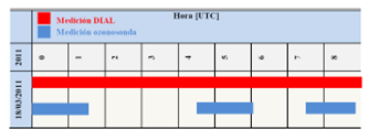
Where   the horizontal red bar indicate the total time of measurement of the DIAL   system and the blue bar indicate the time of flight of the ozonesounding. Can   you show that the DIAL systems was operating more than nine hours. If we select   a time of integration of three hours we can obtain three independent measurements   that each one can be compared with each balloon sonde launched (same period   time of flight). Now we can decrease the time of integration, and we can   derivate for example more profiles.</font></p>     <p><font size="2" face="Verdana">The   advantage using signals obtained by a DIAL system, is that we can use the   signals in 355 nm from the Nd:YAG laser for retrieved a temperature profile   without produced any interference on the ozone measurements.</font></p>     <p><font size="2" face="Verdana">Results   and discussion</font></p>     <p><font size="2" face="Verdana">We   have taken from the total measurement about nine hours from Rayleigh, three   independent period of time which we calculated the temperature profile using a   time of 180 minutes of integration. This time is quasi-coincident with the time   of flight of the ozonesounding launched beside, 1 km away of the DIAL system in   Río Gallegos. This means that we can compare temperature derived from both   instruments.</font></p>     <p><font size="2" face="Verdana">In   Figure 2, we showed the comparison of the temperature profile between the   Rayleigh lidar temperature and the radiosounding.</font></p>     <p><font size="2" face="Verdana"><img width=291 height=242 id="Imagen 4" src="/img/revistas/rbf/v20n20/v20n20a12-image003.png"></font></p>     <p><font size="2" face="Verdana"><img width=287 height=460 id="Imagen 5" src="/img/revistas/rbf/v20n20/v20n20a12-image004.png"></font></p>     <p><font size="2" face="Verdana">
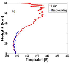
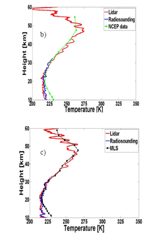
Figure   2. Comparison of the temperature profiles; a), b), c) are the temperature   profile by the Rayleigh lidar (red line) compared with radiosounding (blue   line). b) show the comparison with NCEP data (dashed green line with square)   for March 17, 2011 in Río Gallegos and c) show the comparison with a MLS   sensor(dashed black line with square) aboard AURA-NASA in March 17, 2011 lat=-   51.74 °, lon= -75.23 °, time: 06:03:09 (UTC).</font></p>     <p><font size="2" face="Verdana">The   region of comparison between both instruments is a disvantage due they have   different heights of cover.</font></p>     ]]></body>
<body><![CDATA[<p><font size="2" face="Verdana">In   the case of the Rayleigh lidar we can obtain temperature profile from aprox. 10   km up to 60 km. While in the balloon sonde only we can measured temperature   profile between the surface up to 32 km. The effective zone where both   instruments can be compared, cover the range 10 to 32 km, aprox, limited in the   lower part for the lidar and in the higher part for the balloon burst altitude.</font></p>     <p><font size="2" face="Verdana">The   Figure 2 has shown the good agreement between the diferent profiles, having a   relative error lidar - radiosounding lower than 4 %. Additional in b) we superposed   the NCEP data for the same day of measurement, and c) show the comparison with   the data provided by the MLS instrument aboard the plataform AURA-NASA.</font></p>     <p><font size="2" face="Verdana">CONCLUSION</font></p>     <p><font size="2" face="Verdana">This   paper has shown three independent temperature profiles derivated with a Rayleigh   temperature lidar for one day (March 17, 2011). These profiles were obtained as   a part of the OZITOS II Campaign described above. In each measurement the   Rayleigh temperature profiles were compared with the radiosounding aboard the   balloon sonde. The effective region for the comparison can be established due figure 2 in the region   between 10 up to 30 km aprox. Both instruments have shown good agreement in   this region, with a typical relative error lower than 4 %. We have observed   also that in this night the three lidar profiles are similar, indicating that   the atmospheric conditions were stable. As a comparison with other instrument   as the NCEP data and MLS instrument aboard the AURA-NASA satellite has been to   do it. It measurements were superposed in the profiles b) and c) (figure 2)   showing very good agreement in the region above 20 km. For the region below   both measurements (NCEP data and MLS) indicate a discrepancy very similar when   are compared with the radiosounding and temperature lidar profiles.</font></p>     <p><font size="2" face="Verdana">ACKNOWLEDGMENTS</font></p>     <p><font size="2" face="Verdana">The   authors would like to thank JICA (Japan International Cooperation Agency) by   financial support of UVO3 Patagonia Project; the CNRS in France for their   collaboration in facilitating the shelter and part of the electronic   instruments of DIAL.</font></p>     <p><font size="2" face="Verdana">Analyses   used in this paper were produced with the Giovanni online data system,   developed and maintained by the NASA GES DISC.</font></p>     <p><font size="2" face="Verdana">REFERENCES</font></p>     <!-- ref --><p><font size="2" face="Verdana">1.-   Acker and, J. G., G. Leptoukh, (2007), Online Analysis Enhances Use of NASA   Earth Science Data”, Eos, Trans. AGU, Vol. 88, No. 2, pages 14 and 17.</font>&nbsp;&nbsp;&nbsp;&nbsp;&nbsp;&nbsp;&nbsp;&nbsp;[&#160;<a href="javascript:void(0);" onclick="javascript: window.open('/scielo.php?script=sci_nlinks&ref=229516&pid=S1562-3823201200040001200001&lng=','','width=640,height=500,resizable=yes,scrollbars=1,menubar=yes,');">Links</a>&#160;]<!-- end-ref --><!-- ref --><p><font size="2" face="Verdana">2.-   Gross, M.R., McGee, T.J., Ferrare, R.A., Singh, U.N., Kimvilakani, P, (1997),   Temperature measurements made with a combined Rayleigh–Mie and Raman lidar,   Applied Optics ,36, pp, 5987–5995.</font>&nbsp;&nbsp;&nbsp;&nbsp;&nbsp;&nbsp;&nbsp;&nbsp;[&#160;<a href="javascript:void(0);" onclick="javascript: window.open('/scielo.php?script=sci_nlinks&ref=229517&pid=S1562-3823201200040001200002&lng=','','width=640,height=500,resizable=yes,scrollbars=1,menubar=yes,');">Links</a>&#160;]<!-- end-ref --><!-- ref --><p><font size="2" face="Verdana">3.-   Gu, Y.Y., Gardner, C.S., Castleberg, P.A., Papen, G.C., Kelley, M.C, (1997),   Validation of the lidar in-space technology experiment: stratosphere   temperature and aerosol measurements,Applied Optics, 36, pp, 5148–5157.</font>&nbsp;&nbsp;&nbsp;&nbsp;&nbsp;&nbsp;&nbsp;&nbsp;[&#160;<a href="javascript:void(0);" onclick="javascript: window.open('/scielo.php?script=sci_nlinks&ref=229518&pid=S1562-3823201200040001200003&lng=','','width=640,height=500,resizable=yes,scrollbars=1,menubar=yes,');">Links</a>&#160;]<!-- end-ref --><!-- ref --><p><font size="2" face="Verdana">4.-   Komhyr, W.D., (1969), Electrochemical concentration cells for gas analysis,   Ann. Geoph., 25, 203-210.</font>&nbsp;&nbsp;&nbsp;&nbsp;&nbsp;&nbsp;&nbsp;&nbsp;[&#160;<a href="javascript:void(0);" onclick="javascript: window.open('/scielo.php?script=sci_nlinks&ref=229519&pid=S1562-3823201200040001200004&lng=','','width=640,height=500,resizable=yes,scrollbars=1,menubar=yes,');">Links</a>&#160;]<!-- end-ref --><!-- ref --><p><font size="2" face="Verdana">5.-   Komhyr, W.D., (1971), Development of an ECC- Ozonesonde, NOAA Techn. Rep. ERL   200-APCL 18ARL-149.</font>&nbsp;&nbsp;&nbsp;&nbsp;&nbsp;&nbsp;&nbsp;&nbsp;[&#160;<a href="javascript:void(0);" onclick="javascript: window.open('/scielo.php?script=sci_nlinks&ref=229520&pid=S1562-3823201200040001200005&lng=','','width=640,height=500,resizable=yes,scrollbars=1,menubar=yes,');">Links</a>&#160;]<!-- end-ref --><!-- ref --><p><font size="2" face="Verdana">6.-   Nedeljkovic, D., Hauchecorne, A., Chanin, M.L, (1993), Rotational Raman lidar   to measure the atmospheric- temperature from the ground to 30 km, IEEE   Transactions on Geoscience and Remote Sensing, 31,pp, 90–101.</font>&nbsp;&nbsp;&nbsp;&nbsp;&nbsp;&nbsp;&nbsp;&nbsp;[&#160;<a href="javascript:void(0);" onclick="javascript: window.open('/scielo.php?script=sci_nlinks&ref=229521&pid=S1562-3823201200040001200006&lng=','','width=640,height=500,resizable=yes,scrollbars=1,menubar=yes,');">Links</a>&#160;]<!-- end-ref --><!-- ref --><p><font size="2" face="Verdana">7.-   Steinbrecht, W., and A.I. Carswell, (1995), Evaluation of the effect of Mount   Pinatubo aerosol on differential absortion lidar measurements of stratospheric   ozone. J.Geophys. Res.100, 1215-1233.</font>&nbsp;&nbsp;&nbsp;&nbsp;&nbsp;&nbsp;&nbsp;&nbsp;[&#160;<a href="javascript:void(0);" onclick="javascript: window.open('/scielo.php?script=sci_nlinks&ref=229522&pid=S1562-3823201200040001200007&lng=','','width=640,height=500,resizable=yes,scrollbars=1,menubar=yes,');">Links</a>&#160;]<!-- end-ref --><p><font size="2" face="Verdana">8.-   Wolfram, A. E., J. Salvador, R. D’Elia, C. Casiccia, N. Paes Leme, A. Pazmiño,   J. Porteneuve, S. Godin-Beekman, H. Nakane and E. J. Quel, (2008), New   Differential absorption lidar for stratospheric ozone monitoring in Patagonia,   south Argentina, J. Opt. A: Pure Appl. Opt. 10, 104021 (7pp).   oi:10.1088/1464-4258/10/10/104021.</font></p>      ]]></body><back>
<ref-list>
<ref id="B1">
<label>1</label><nlm-citation citation-type="journal">
<person-group person-group-type="author">
<name>
<surname><![CDATA[Leptoukh]]></surname>
<given-names><![CDATA[J. G., G.]]></given-names>
</name>
</person-group>
<article-title xml:lang="en"><![CDATA[Online Analysis Enhances Use of NASA Earth Science Data]]></article-title>
<source><![CDATA[Eos, Trans. AGU]]></source>
<year>2007</year>
<volume>88</volume>
<numero>2</numero>
<issue>2</issue>
<page-range>14 and 17</page-range></nlm-citation>
</ref>
<ref id="B2">
<label>2</label><nlm-citation citation-type="">
<person-group person-group-type="author">
<name>
<surname><![CDATA[Gross]]></surname>
<given-names><![CDATA[M.R.]]></given-names>
</name>
<name>
<surname><![CDATA[McGee]]></surname>
<given-names><![CDATA[T.J.]]></given-names>
</name>
<name>
<surname><![CDATA[Ferrare]]></surname>
<given-names><![CDATA[R.A.]]></given-names>
</name>
<name>
<surname><![CDATA[Singh]]></surname>
<given-names><![CDATA[U.N.]]></given-names>
</name>
<name>
<surname><![CDATA[Kimvilakani]]></surname>
<given-names><![CDATA[P]]></given-names>
</name>
</person-group>
<source><![CDATA[Temperature measurements made with a combined Rayleigh-Mie and Raman lidar: Applied Optics]]></source>
<year>1997</year>
<volume>36</volume>
<page-range>5987-5995</page-range></nlm-citation>
</ref>
<ref id="B3">
<label>3</label><nlm-citation citation-type="">
<person-group person-group-type="author">
<name>
<surname><![CDATA[Gu]]></surname>
<given-names><![CDATA[Y.Y.]]></given-names>
</name>
<name>
<surname><![CDATA[Gardner]]></surname>
<given-names><![CDATA[C.S.]]></given-names>
</name>
<name>
<surname><![CDATA[Castleberg]]></surname>
<given-names><![CDATA[P.A.]]></given-names>
</name>
<name>
<surname><![CDATA[Papen]]></surname>
<given-names><![CDATA[G.C.]]></given-names>
</name>
<name>
<surname><![CDATA[Kelley]]></surname>
<given-names><![CDATA[M.C]]></given-names>
</name>
</person-group>
<article-title xml:lang="en"><![CDATA[Validation of the lidar in-space technology experiment]]></article-title>
<source><![CDATA[stratosphere temperature and aerosol measurements: Applied Optics]]></source>
<year>1997</year>
<volume>36</volume>
<page-range>5148-5157</page-range></nlm-citation>
</ref>
<ref id="B4">
<label>4</label><nlm-citation citation-type="journal">
<person-group person-group-type="author">
<name>
<surname><![CDATA[Komhyr]]></surname>
<given-names><![CDATA[W.D.]]></given-names>
</name>
</person-group>
<source><![CDATA[Electrochemical concentration cells for gas analysis, Ann. Geoph.]]></source>
<year>1969</year>
<volume>25</volume>
<page-range>203-210</page-range></nlm-citation>
</ref>
<ref id="B5">
<label>5</label><nlm-citation citation-type="">
<person-group person-group-type="author">
<name>
<surname><![CDATA[Komhyr]]></surname>
<given-names><![CDATA[W.D.]]></given-names>
</name>
</person-group>
<source><![CDATA[Development of an ECC- Ozonesonde, NOAA: Techn. Rep. ERL 200-APCL 18ARL-149]]></source>
<year>1971</year>
</nlm-citation>
</ref>
<ref id="B6">
<label>6</label><nlm-citation citation-type="journal">
<person-group person-group-type="author">
<name>
<surname><![CDATA[Nedeljkovic]]></surname>
<given-names><![CDATA[D.]]></given-names>
</name>
<name>
<surname><![CDATA[Hauchecorne]]></surname>
<given-names><![CDATA[A.]]></given-names>
</name>
<name>
<surname><![CDATA[Chanin]]></surname>
<given-names><![CDATA[M.L]]></given-names>
</name>
</person-group>
<article-title xml:lang="en"><![CDATA[Rotational Raman lidar to measure the atmospheric- temperature from the ground to 30 km]]></article-title>
<source><![CDATA[IEEE Transactions on Geoscience and Remote Sensing]]></source>
<year>1993</year>
<volume>31</volume>
<page-range>90-101</page-range></nlm-citation>
</ref>
<ref id="B7">
<label>7</label><nlm-citation citation-type="journal">
<person-group person-group-type="author">
<name>
<surname><![CDATA[Steinbrecht]]></surname>
<given-names><![CDATA[W.]]></given-names>
</name>
<name>
<surname><![CDATA[Carswell]]></surname>
<given-names><![CDATA[A.I.]]></given-names>
</name>
</person-group>
<article-title xml:lang="en"><![CDATA[Evaluation of the effect of Mount Pinatubo aerosol on differential absortion lidar measurements of stratospheric ozone]]></article-title>
<source><![CDATA[J.Geophys. Res.]]></source>
<year>1995</year>
<volume>100</volume>
<page-range>1215-1233</page-range></nlm-citation>
</ref>
<ref id="B8">
<label>8</label><nlm-citation citation-type="journal">
<person-group person-group-type="author">
<name>
<surname><![CDATA[Wolfram]]></surname>
<given-names><![CDATA[A. E.]]></given-names>
</name>
<name>
<surname><![CDATA[Salvador]]></surname>
<given-names><![CDATA[J.]]></given-names>
</name>
<name>
<surname><![CDATA[D’Elia]]></surname>
<given-names><![CDATA[R.]]></given-names>
</name>
<name>
<surname><![CDATA[Casiccia]]></surname>
<given-names><![CDATA[C.]]></given-names>
</name>
<name>
<surname><![CDATA[Paes Leme]]></surname>
<given-names><![CDATA[N.]]></given-names>
</name>
<name>
<surname><![CDATA[Pazmiño]]></surname>
<given-names><![CDATA[A.]]></given-names>
</name>
<name>
<surname><![CDATA[Porteneuve]]></surname>
<given-names><![CDATA[J.]]></given-names>
</name>
<name>
<surname><![CDATA[Godin-Beekman]]></surname>
<given-names><![CDATA[S.]]></given-names>
</name>
<name>
<surname><![CDATA[Nakane]]></surname>
<given-names><![CDATA[H.]]></given-names>
</name>
<name>
<surname><![CDATA[Quel]]></surname>
<given-names><![CDATA[E. J.]]></given-names>
</name>
</person-group>
<article-title xml:lang="en"><![CDATA[New Differential absorption lidar for stratospheric ozone monitoring in Patagonia, south Argentina]]></article-title>
<source><![CDATA[J. Opt. A: Pure Appl. Opt.]]></source>
<year>2008</year>
<volume>10</volume>
<page-range>7</page-range></nlm-citation>
</ref>
</ref-list>
</back>
</article>
