ARTICLE ACADEMIC

 

Response to a financial crisis in Argentina: How to deal
with wealth inequality

 

Respuestas a crisis financieras en Argentina: Como lidiar
con la desigualdad

 

 

Pablo Matías Herrera^ρ , Javier García Fronti^£
ρ Universidad de Buenos Aires, Facultad de Ciencias Económicas, CIMBAGE (IADCOM), Ciudad
Autónoma de Buenos Aires, Argentina, pablomatiasherrera@gmail.com
^£ Universidad de Buenos Aires, Facultad de Ciencias Económicas, CIMBAGE (IADCOM), Ciudad
Autónoma de Buenos Aires, Argentina, javier.garciafronti@economicas.uba.ar
Recepción:  02/01/2019       Aceptación: 19/03/2019

 

 

---

Abstract

Ten years from the last financial crisis, and 17 years from the most virulent one in the history of Argentina, its government insists on policies that spark exchange rate volatility in attempting to right macroeconomic imbalances. The effects of this volatility on inequality should not be ignored as, for the most part, structural reform must be socially sustainable as well as economically sustainable.

This work analyses some aspects of the response of the government to the 2018 financial crisis in Argentina. To do this, this work is organized in three sections. The first section gives a general overview of the current crisis and the response of the government and its distributive effects. The second section analyses a model and extends it for the case of an economy with two sectors, one of which has access to the world market, the effects of changes in the exchange rate on inequality are analysed and calibrated for Argentina focusing on the parameter τ. Finally, some policy recommendations are proposed.

Keywords: Financial crisis response, wealth inequality, tax structure

---

Resumen

A 10 años de la última crisis financiera, y a 17 de la crisis económica más virulenta de Argentina, su gobierno insiste con políticas que generan volatilidad en el tipo de cambio con el objetivo de subsanar desbalances macroeconómicos. Las reformas estructurales deben ser sustentables tanto desde el punto de vista macroeconómico como social y, por lo tanto, los efectos de esta volatilidad sobre la desigualdad social no deben ser ignorados.

Este trabajo analiza algunos aspectos de la respuesta oficial a la crisis financiera Argentina. Para llevar a cabo este objetivo, el trabajo se divide en tres partes. La primera parte expone un breve resumen de la crisis financiera actual, la respuesta del gobierno, y sus impactos distributivos. La segunda parte analiza un modelo de desigualdad y lo extiende al caso de una economía de dos sectores, uno de los cuáles tiene acceso al mercado mundial externo. Se analizan los efectos de cambios en el tipo de cambio sobre la desigualdad en esta economía y luego se calibra el modelo para el caso de Argentina. Finalmente, se exploran algunas recomendaciones de política.

Palabras clave: Respuestas a crisis financieras, desigualdad, estructura impositiva.

---

Clasification JEL: H12, H23.

---

 

 

1. Introduction

A parity with the dollar (called “Convertibilidad”) was established in Argentina during 1991, with good economic results during the first half of that decade. However, from 1997 onwards, this monetary policy has been accompanied by a deep economic recession. In 1999 Fernando de la Rúa assumes the presidency. Under his mandate, poverty increased up to 35.4 percent in October 2001. Despite government attempts to maintain the fixed exchange rate regime, external factors and high local interest rates, forced the resignation of the president in December 2001, see (García-Fronti, Miller, & Zhang, 2002). Poverty continued to rise and reached 49.7 percent in May 2002.

In May of 2003, Néstor Kirchner assumes the presidency. His tenure was characterized by favourable international economic conditions and policy measures aiming social welfare. Annual economic growth levels were, in average, of 8.5 percent, the poverty level was reduced to 26 percent. In December 2007, Cristina Fernández de Kirchner became president (Levitsky & Murillo, 2008). The first of its mandates was characterized by an annual growth of 3.5 percent on average. However, her second term ended with macroeconomic imbalances, a weakened institutional framework and unreliable official statistics.

With large fiscal deficits, foreign exchange controls, high inflation, low investment, price controls, regressive subsidies, trade restrictions and capital control, in December 2015, Mauricio Macri assumes the presidency. Among its first measures, he eliminated exchange controls and adopted a flexible exchange rate regime, initiating the process of realignment of the prices of public services and the reduction of subsidies. The Government also initiated structural reforms to strengthen the competitiveness of the economy and eliminate distortions in the private sector, including the reduction of export taxes and the relaxation of import controls. One important achievement was the recovery of public trust in official statistics. However, all these measures were carried out with the explicit purpose of attracting foreign capitals, without considering the negative impact to poverty reduction and income distribution.

During the first years of the Macri government, external vulnerabilities have been increasing. Opening of imports and the appreciation of the peso, increased the current account deficit in 2016-2017. Fiscal year 2018 began with a severe drought that had a great impact on agricultural production and exports inside Argentina and with an international negative context marked by more restrictive global financial conditions due to a rise in US interest rates. In this context, in April, a group of investors unexpectedly withdrew thousands of millions of dollars, resulting in a large depreciation of the peso Moreover, investors expressed concern regarding the renewal of the Central Bank's short-term debt (LEBAC) and the increase in the sovereign risk premium.

With the aim of restoring market confidence, the Argentine government requested financial assistance from the International Monetary Fund (IMF) and an agreement was reached in July. After a relatively quiet period, at the end of August, there was a new round of global financial turmoil, marked by the depreciation of the Turkish lira in three days. During the generalized depreciation of emerging market currencies, the Argentine peso was the most affected, accumulating a depreciation of 50 percent so far this year. In this context President Macri announced a stronger fiscal adjustment to reduce financing needs, aiming to restore investors’ confidence. The main announcement, considering that the export sector has obtained exceptional rents due to the depreciation of the peso, was the application of export taxes.

Ten years after the last global financial crisis, the current Argentine government continues to resort to an orthodox formula to curb exchange rate volatility. To alleviate the social situation, the IMF asked to monitor the situation and encourage national authorities to design a protection strategy to cover vulnerable population. However, all these measures ignore the fact that, in our opinion, Argentina's main problem is inequality, therefore policies should aim for a serious redistribution of income, see (Lustig, Lopez-Calva, & Ortiz-Juarez, 2012). The tax reform launched by the government, which includes a new export tax, is more of a tax package since it does not imply fundamental structural changes.

This work proposes an analysis of some aspects of government response to the current financial crisis. Our working hypothesis is that the current wealth dynamic in Argentina tends to a more unequal wealth distribution, which should be countered by policy actions. We test this by the calibration of a formal model to empirical data. The following section presents a formal tool that allows us to explore how the government should respond to the crisis from a public welfare point of view. This tool is a two-sector economy where a mechanism of wealth transfer operates between individuals. In the third section, the proposed model is calibrated, and we simulate different scenarios for Argentina. Some preliminary proposals on how to respond to a financial crisis in the context of Argentina as a conclusion.

 

2. The Model

To understand some aspects of the macroeconomic context previously exposed, this section proposes a formal tool for policymakers that allows to understand different responses to financial crises, considering negative impacts on wealth distribution. Personal wealth has been studied by empirical works such as (Piketty, Saez, & Zucman, 2017; Saez & Zucman, 2016), and, from the theoretical point of view^†, (Cagetti & De Nardi, 2008; De Nardi, 2015). Moreover, there’s a more parsimonious econophysics literature, which sometimes take the form of networks models (Benisty, 2017; Liu & Serota, 2018). Within this view we choose a framework which is the simplest framework that can reproduce a credible wealth distribution of an economy.

The proposed tool is an extension of the model published by Berman, Peters and Adamou (Berman, Peters, & Adamou, 2016). The authors model the wealth of an individual  as a geometric Brownian motion with a correction that represents interaction between individuals of a given economy, and the stochastic differential equation which personal wealth must follow is given by (we have slightly changed the original notation):

The first term of Eq. (1) represents the instant variation on wealth under no taxation and the second term could be thought as a common pot from which everyone contributes according to wealth and receives according to the size of the pot (because both transferences are simultaneous, τ is unconstrained). N is the size of the ensemble, E_N[.] is the ensemble in average µ,σ and τare real constants, and dB_i is the increment of a simple Brownian motion.

Different values for τ implies different regimes for the dynamics of personal wealth. Positive values for τ indicate progressive transferences of wealth (net transferences from individuals with wealth greater than E_N[w] to everyone else), with the terminal distribution of wealth (T → ∞) converging to an inverse gamma distribution, see (Berman, Peters, & Adamou, 2017).

The parameter τ =  0 implies the traditional (Black & Scholes, 1973). Under this regime, the time t distribution of wealth is lognormal with mean µt and variance σ²t (see, for example (Lin, 2006)). This regime implies that the wealth of any given individual is non-negative, and, unlike the first case, that no stationary distribution exists. In fact, the limit for T → ∞ of any given trajectory is 0, the difference between the behaviour of the ensemble and individual trajectories under the long-time limit is due to the non-ergodic nature of the model. Finally, for τ < 0 we have regressive net transfer of wealth and, as was the case before, no stationary distribution. The difference with the previous regime is that individual wealth can be negative and typically is.

The dynamics induced by different regimes are quite different and this makes the model very flexible, allowing to infer the general tendency of the economy by calibrating τ to reproduce the empiric distribution of wealth and generating different scenarios via simulation (for any values of the parameters µ,σ and τ). Yet this model, as any other, has a space of application in which its assumptions are reasonable. We focus on two key assumptions.

Firstly, the model assumes everyone has access to the same average rate of growth, µ. This is perfectly reasonable in economies with well-developed capital markets. However, in economies with a dual productive structure, where a small high productivity sector linked to the world market coexists with a large low-productivity sector associated with internal market, there are different values of µ.

Secondly, it should be noted that τ is a very high-level parameter, this is, it represents any and all interactions between individuals, including although not restricted to those interactions between the public and private sector, most notably those relations mediated by the system of taxes and subsidies. In an economy with an important percentage of its population outside the formal sector, or alternatively in economies. Alternatively, the distinction between sectors could be merely temporary, large fluctuations in the foreign exchange rate could trigger large changes in the relative prices of an economy, and particularly, large fluctuations in return on investment linked to the world and domestic markets. This effect could be sufficiently lasting or large that the public sector decides to intervene. This intervention would and should be asymmetric and, in this scenario, τ would be too high level to reflect or properly model this intervention.

With this in mind, this extension consider a partition of the population in two sectors N = N₁ + N₂ where individuals of sector 1 have access (permanent or temporary) to the average wealth growth rat µ₁, while individuals of sector 2, have access to the rate µ₂ where µ₁ ≠ µ₂, and suppose without loss of generality that µ₁< µ₂. Subscript individuals from sector 1 as i = 1,2,...,N₁, and individuals of sector 2 as j = N₁ + 1,...,N, the wealth of individuals (i,j) follows:

Where µ_i is the average ensemble growth rate for sector N_i , and τ_i is the wealth transference rate for sector N_i. Note that there ar different distribution of wealth between sectors altogether and could be transferences of wealth between sectors. This wealth dynamic implies that everyone contributes to a common pot, according to wealth (at differential rates) and receives according to the size of the pot. For example, values τ₁ = τ₂ = τ > 0 implies wealth transference from sector 2 to 1, as well as from rich to poor.  As we will see in the next section, for a range of values of τthe resulting distribution is multimodal and might be reasonable to model two economies that transfer wealth among each other. Next section studies different regimes running simulation exercises.

 

3. Simulation and Estimation

The model specification presents several regimes, some of which are useful to explore what could happen in an economy given (induced) changes in τ_i, by the government. In this section we simulate scenarios, we estimate the values of (µ₁, µ₂, σ) and we calibrate (τ₁,τ₂₎ to Argentina. The resulting wealth distribution resembles the empirical one in the best way possible given the constraints on the available data.

For the simulations we take, unless otherwise specified, an economy with population size of N = 1500, of which N₁ = 1000, initial time t₀, terminal time T = 10 years, and time step years^‡. To simulate the system od stochastic differential equations given by (Eq. (2)) we use Euler-Maruyama numerical scheme (see, for example (Higham, 2001)). This means that we approximate (Eq. (2)) as:

As the parameters of interest are τ₁,τ₂ we take them as variable and fix µ₁ = 0.05, µ₂ = 0.1 and σ = o.5 ^§. For each parameter we study five configurations, namely that τ_i > µ_i, µ_i > τ_i, > 0, -µ_i < τ_i < 0, -µ_i > τ_i , and τ_i = µ_i, which roughly translates to τ_i is positive, very positive, negative, very negative, or equal to the ensemble growth rate. We identify the same regimes as in (Berman et al., 2016) (previously explained in section 2): (C1) both (τ_1,τ₂) are positive (C2) are both negative and (C3) the parameters change signs.

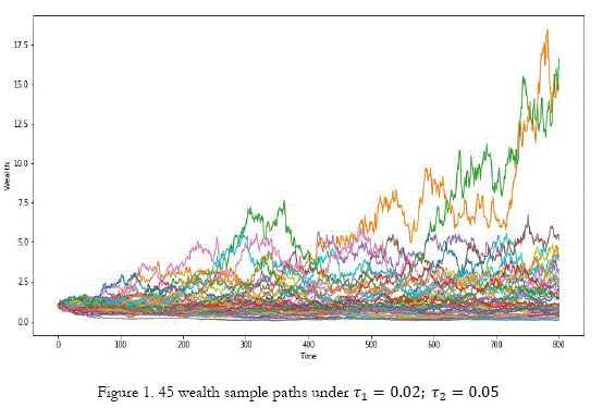
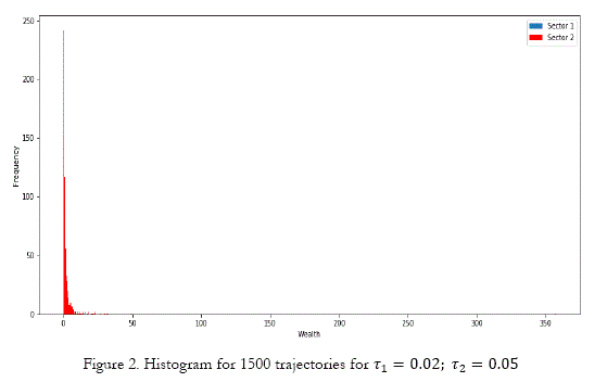
Case 1 (C1) happens when both τ_i > 0. For small values of τ_i (i.e. τ_i < µ_i) we have a dynamic like GBM. All wealth paths are non-negative with the occasional lucky trajectory growing much faster than the rest and pushing the ensemble average above most trajectories (figure 1) which are concentrated near the zero. As expected the resulting distribution is (figure 2) resembles both the inverse gamma (the stationary distribution in (Berman et al., 2016) under τ > 0) and lognormal (the distribution under τ_i = 0 ) distributions. Also, all outliers corresponding to a large terminal wealth belong to sector 2 even though τ₂ > τ₁.

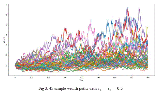
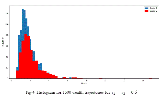
If τ_i is greater than µ_i, while the majority of trajectories still have terminal wealth near zero, we have a much more even distribution of personal wealth trajectories (figure 3). Maximum wealth is also much lower than in the former case ($16 vs. $350) and the corresponding histogram is in figure 4. Moreover, very high wealth outliers belong to both sectors.

Between τ_i < µ_i, and τ_i > µ_i we have 0 < τ_j≤ µ_j, τ_k≥ µ_k, j ≠ k. The results for these cases are omitted for reasons of space, but the resulting wealth distribution lie within fig.2 and fig.4 where outliers for maximal wealth tend to belong to the sector with τ_j≤ µ_j, this is, the sector that contributes proportionally a smaller fraction of its wealth to redistribution (and also receives less) so its dominated by “lucky” trajectories.

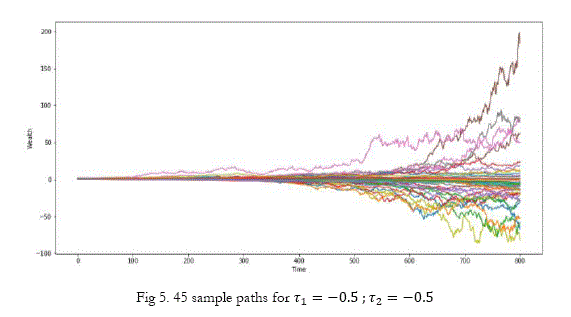
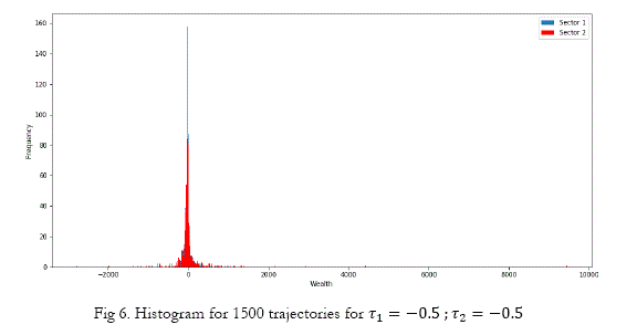
Case 2 (C2) happens when τ_i < 0. Now wealth trajectories can decrease without bound, and some trajectories do, while others increase without bound (figure 5). The resulting distribution is symmetric centred around zero and very highly frequency around the mode (figure 6), an experiment with increasing terminal time suggests that the limiting distribution (when excluding outliers) is degenerate. The distinction between |τ_i | > µ_i  and |τ_i |< µ_i here is uninteresting.}

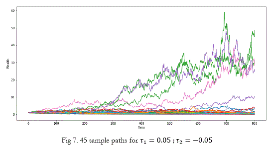
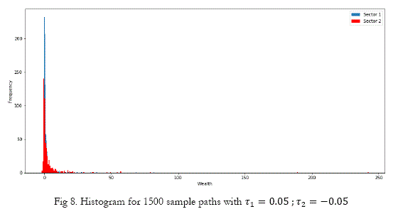
Case 3 (C3) happens when τ_i change signs and is the most versatile as its resulting dynamic lies between C1 and C2. For small absolute values of τ_i we have some wealth paths going negative yet not without bound (figure 7 and figure 8), which is interesting because it would not be reasonable to observe net personal wealth tending to -∞ in a real world economy because of bankruptcy laws, but it would be to see a small fraction of individuals to have finite and small negative net worth because of debt outgrowing assets. A similar dynamic result from having 0 < τ_i < µ_i, τ_j < -µ_j, but this is more similar to C2 in the sense that wealth can decrease without bound.

Once identified the regimes of the model we proceed to its calibration to Argentina. The dataset is composed of tax collection data from the local tax agency namely, the Aministración federal de ingresos públicos (AFIP) on a net worth tax named bienes personales, which distinguishes between domestic (sector 1) and external assets (sector 2). The periodicity of the data is annual and ranges from 2007 to 2016 fiscal years. For the estimation of the volatility parameter, σ, we took the “Mercado de Valores de Buenos Aires” (MERVAL) index as indicative of the whole economy. Finally, the number for the population of adults each year come from the national statistics institute (Instituto nacional de estadística y censos).

We follow the uncontroversial estimation strategy of parameters (µ₁,µ₂,σ) as in (Berman et al., 2016) as explained next. We suppose that the average individual wealth grows exponentially at the same rate as the ensemble, i.e. sector_i = e^µi(t-t0). We estimate µ_i via least squares linear regression on the natural logarithm of both sides of the equation. The σ parameter is estimated as the standard deviation of historical log-returns on the MERVAL index (argentine stock index) for the last year (November 2017-18) and scale it appropriately. The point estimates of the parameters are µ₁ = 0.27, µ₂ = 0.32, and σ = 0.395. This are reasonable values for the period considering the inflationary process as described in the first section. An important point is that µ₂ > µ₁, also with the recent developments regarding the exchange rate of the peso, and lower domestic demand due to the current recession would increase this differential in average growth rates.

Finally for the policy parameters (τ₁, τ₂), they are calibrated so as to minimize the squared difference between the observed wealth distribution quantile (we take this to be the percentage of the adult population that is reached by our chosen net worth tax, which is 6.7% on average in our case) and the theoretical quantile produced by the model. We use the algorithm presented in (Nelder & Mead, 1965) for the minimization, and rescale observed wealth so that total observed wealth for t₀ = 2007  is equal to $1.

The optimization process produces the values of τ₁ = 0.16313025, and τ₂ = -0.05111769 for the whole period. Given the constraints on the data, this value should be taken only as indicative of the real values, which are unknown. With this caveat in mind, this specification lies under C3 and its dynamics are like fig.7 (small positive τ₁ < 0.27, and small negative τ₂). Therefore, a policy maker seeking to reduce wealth inequality would try to transition from the dynamics as given by C3 to those given by C1 by increasing τ₂.

This could take many forms, the most direct being tax policies. A direct tax on individual wealth is sure to decrease wealth inequality at an uncertain cost in future growth rates. A tax on very high wealth outliers from the external sector and a corresponding redistribution, perhaps within the same sector would also diminish inequality but make the external sector less appealing for business and so deter investors. Both a careful study of the determinants of τ_i, together with awareness on the macroeconomic effects of changes in tax legislation is needed to give more concrete policy recommendations.

 

Conclusion(s)

Ten years after the last global financial crisis, the current argentine government continues to resort to orthodox formulas to deal with local financial crisis, ignoring income inequalities. This work analysed some aspects of Argentina's response to the current financial crisis. To do so, in the first section a summary of the macroeconomic and social context of the last years of the country was presented. It concluded that the tax reforms carried out by the last government do not imply substantive structural changes and that the only way to make the country viable is to make a project based on greater equality. In the second section a formal tool named RGBM was presented, followed by the proposal of an extension that include mechanisms of wealth transfer. In the third section, the proposed model was calibrated and the trend of the distribution of wealth was analysed based on the variation of wealth transfer rates.

The calibration of the model for Argentina indicates that it is in CASE 3 (changes of signs) and its dynamics are like fig.7 (small positiveτ₁ < 0.27, and small negative τ₂). Therefore, to reduce wealth inequality, a policymaker must transform the dynamics from CASE 3 to CASE 1, by increasing τ₂. This could be tax on very high wealth outliers (external sector).

Some future lines of research include improving the estimation of the wealth distribution by considering alternative data sources, as well as a wider time window, complementing the simulation exercise with an analytical study of the statistical properties of the proposed model and the study of the determinants of wealth transfer rates.

 

Notas

^† The mainstream framework relies on general equilibrium with heterogenous agents (either infinitely-lived agents or in an overlapping generation context).

^‡ The decision on the values of N, and dt is motivated by its computational cost, the decision on T is motivated on a long, yet relevant terminal time for a human adult population.

^§ This parameter values are arbitrary and aim to clearly define the regimes given the values of N and T rather than being indicative of any real world economy in particular.

 

References

Benisty, H. (2017). Simple wealth distribution model causing inequality-induced crisis without external shocks. Physical Review E, 95(5), 052307.        [ Links ]

Berman, Y., Peters, O., & Adamou, A. (2016). Far from equilibrium: Wealth reallocation in the United States. ArXiv Preprint ArXiv:1605.05631.        [ Links ]

Berman, Y., Peters, O., & Adamou, A. (2017). An Empirical Test of the Ergodic Hypothesis: Wealth Distributions in the United States.        [ Links ]

Black, F., & Scholes, M. (1973). The Pricing of Options and Corporate Liabilities. Journal of Political Economy, 81, 637–654.        [ Links ]

Cagetti, M., & De Nardi, M. (2008). Wealth inequality: Data and models. Macroeconomic Dynamics, 12(S2), 285–313.        [ Links ]

De Nardi, M. (2015). Quantitative models of wealth inequality: A survey. National Bureau of Economic Research.        [ Links ]

García-Fronti, J., Miller, M., & Zhang, L. (2002). Sovereign default by Argentina:’slow motion train crash’or self-fulfilling crisis? CEPR Discussion Paper, 3399, 1–17.        [ Links ]

Higham, D. J. (2001). An algorithmic introduction to numerical simulation of stochastic differential equations. SIAM Review, 43(3), 525–546.        [ Links ]

Levitsky, S., & Murillo, M. V. (2008). Argentina: From kirchner to kirchner. Journal of Democracy, 19(2), 16–30.        [ Links ]

Lin, X. S. (2006). Introductory stochastic analysis for finance and insurance (Vol. 557). John Wiley & Sons.        [ Links ]

Liu, Z., & Serota, R. (2018). On absence of steady state in the Bouchaud–Mézard network model. Physica A: Statistical Mechanics and Its Applications, 491, 391–398.        [ Links ]

Lustig, N., Lopez-Calva, L. F., & Ortiz-Juarez, E. (2012). Declining inequality in Latin America in the 2000s: the cases of Argentina, Brazil, and Mexico. The World Bank.        [ Links ]

Nelder, J. A., & Mead, R. (1965). A simplex method for function minimization. The Computer Journal, 7(4), 308–313.        [ Links ]

Piketty, T., Saez, E., & Zucman, G. (2017). Distributional national accounts: methods and estimates for the United States. The Quarterly Journal of Economics, 133(2), 553–609.        [ Links ]

Saez, E., & Zucman, G. (2016). Wealth inequality in the United States since 1913: Evidence from capitalized income tax data. The Quarterly Journal of Economics, 131(2), 519–578.        [ Links ]