ARTÍCULOS ACADÉMICOS

 

Granularity of the business cycle fluctuations: The Spanish case

 

Omar Blanco Arroyo*, Simone Alfarano**
*Department of Economics, Universitat Jaume I Email:blancoo@uji.es
**Department of Economics, Universitat Jaume I Email:alfarano@eco.uji.es
Recepción: 09/11/2016  Aceptación: 28/12/2016

 

 

---

Abstract:

Following the approach proposed by Gabaix (2011), this paper aims to verify the existence of granularity in the Spanish business cycle fluctuations. A granular firm is characterized by the fact that its idiosyncratic shocks have a significant impact on GDP growth fluctuations. Despite the fact that granular firms constitute just a marginal fraction of the total number of firms, they account for a significant part of business cycle fluctuations. Our analysis shows that half of the GDP growth fluctuations of the Spanish economy can be linked to the idiosyncratic shocks of the largest 100 Spanish firms. Our work contributes to strengthening the empirical relevance of the granular hypothesis. The results show that the Spanish economy, as happens in the US economy, may be represented by a large number of small and medium enterprises whose individual evolution has no impact at the aggregate level, and a small number of large firms whose fluctuations contribute significantly to the variability of the Spanish business cycle.

Keywords: granularity, granular economy, idiosyncratic shocks, aggregate fluctuations, power law behaviour.

---

Clasificación Jel: E32, C16.

---

 

 

Introduction

In mainstream macroeconomics idiosyncratic shocks to firms average out in the aggregate (Lucas, 1977), contributing just marginally to economic fluctuations. Within this framework, shocks affecting the economy have to be exogenous and systemic (i.e. at the level of the whole economy) to generate the business cycle fluctuations with the characteristics that we observe in real data. A classic example is the Real Business Cycle (RBC) model developed by Kydland and Prescott (1982), where the technological shocks affecting the Total Factor Productivity (TFP) generate the characteristics of the business cycle similar to the empirical data. Within this framework, the economy is described by means of a representative consumer and a representative firm acting rationally based upon model-consistent expectations, i.e. rational expectations, when they take decision on their inter-temporal economic plans. The representative agent approach implicitly assumes the existence of a certain level of homogeneity among firms acting in the real world, so that the representative firm meaningfully describes a sort of average firm.

The homogeneity hypothesis has been recently challenged by the empirical work of Gabaix (2011), who explicitly test on what extent firms' idiosyncratic shocks can describe aggregate fluctuations. Gabaix has demonstrated empirically that idiosyncratic shocks to large firms have a significant impact on the business cycle fluctuations of United States, accounting approximately one third of GDP fluctuations. The main idea rest on recognising that the level of heterogeneity of firms' size is so high that cannot be cast into a representative firm approach.

Aggregate fluctuations, therefore, cannot be explained as the sum of small diffusive shocks affecting each and every firm, as it is assumed within the RBC framework. Instead, they can be partially attributed to well identified "grains", which are some of the large firms. If an economy is characterised by this behaviour, it is defined as "granular economy".

The insight of an economy as a granular system deeply questions the conventional macroeconomic approach. It poses new problems to understand the macroeconomic dynamics and new potential implications regarding the application of policies to stabilise the economic cycle (Carvalho and Grassi, 2015). Gabaix (2011) has considered the granular nature of GDP, but other studies have found a granular behaviour in other macroeconomic variables, such as exports (del Rosal, 2013; Di Giovanni and Levchenko, 2012), or even in sectors, such as banking (Blank et al., 2009) or manufacturing (Wagner, 2012).

The aim of this paper is to check whether the granular hypothesis is a characteristic of the Spanish economy, i.e. whether a relevant part of the Spanish business cycle variability may be related to the idiosyncratic shocks of few Spanish large firms. The period under study ranges from 1999 to 2014, a lapse of time of 16 years. In this period Spain experienced a complete business cycle. The expansion phase began in 1995 with the entry of Spain in the Monetary Union. Because of low interest rates and the absence of ex-change rate risk, Spain experienced a sharp increase in the access to credit (Fernandez-Villaverde et al., 2013), which subsequently led to an increase in consumption and investments. One of the sectors that attracted more investments was the real estate sector, which time after would develop a bubble that ended in 2008 as a consequence of the global financial crisis. From 2008 to 2013 Spain suffered the worst recession of its recent history. The last years are instead characterised by a strong GDP growth, particularly in consumption and export.

Spain, therefore, constitutes an interesting case of study for testing the granular hypothesis. As a first step Fig. 1 shows the sum of sales of the top 50 and 100 firms as a fraction of GDP. As one can see, the top 50 firms of the sample account on average for 25% of GDP and top 100 account for 32%. Considering this simple empirical calculation and taking into account that the total number of firms is roughly 3 million***, one can infer the existence of an enormous heterogeneity in the size of the Spanish firms. The question that raises is whether the level of heterogeneity among firms is sufficiently high to generate "granular" macroeconomic fluctuations. The 100 largest firms account just for a marginal fraction of the total number of firms in the economy (0.01% of the total number of firms). Nevertheless, our calculations suggest that the fluctuations of the top 100 Spanish firms, are responsible for approximately half of the GDP growth fluctuations. We can conclude, then, that the Spanish economy is granular.

This paper is organised as follows. Section 2 exposes the data set used in order to carry out the empirical analysis. Section 3 is devoted to the analysis of the type of theoretical distribution that better characterise the empirical firm's size distribution. Section 4 provides a calibration of the baseline model, indicating that the effects are of the right order of magnitude to account for the empirical macroeconomic fluctuations. Section 5 carries out the empirical analysis, where it is shown that the granular residual explains a significant fraction of GDP fluctuations. Finally, section 6 concludes.

 

2. Data set

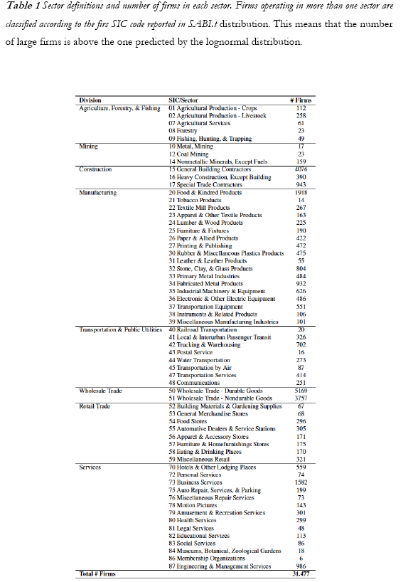
The data set employed in order to carry out the analysis has been taken from SABI (Sistemas de Análisis de Balances Ibéricos), which is a database of Bureau Van Dijk. The initial sample is made up 36.474 firms, with the following entries: volume of sales (S), number of employees (E) and SIC code†††. However, some of the firms in the sample are affected by well identified exogenous shocks, as it is the case of firms that belong to sectors related to hydrocarbons (SIC codes 13, 28 and 29), energy (SIC code 49) and finance (SIC codes 60 and 69). For those firms it might be relatively more difficult to estimate idiosyncratic shocks, since their shocks are mainly exogenous. Therefore, taking into account that these firms could lead to a distortion in the results, they have not been considered, following the original work of Gabaix (2011). After a process of filtering using the SIC code, the number of firms under study is 31.477. Table 1 shows the number of firms that belong to each sector. As it can be seen, there are 61 sectors considered, this allows us to have a representative sample of the Spanish economy. Sectors with the larger numbers of firms are: Wholesale Trade -Durable Goods, Wholesale Trade - Nondurable Goods, General Building Contractors and Food & Kindred Products.

 

3. Empirical distribution of firm size

In order to identify whether the Spanish economy is granular, we have to statistically characterise the empirical distribution of the size of the firms in our sample. We have to precisely quantify the degree of heterogeneity among firms since it is a crucial determinant to compute the level of aggregate fluctuations of GDP, as we will see in the section 4.

3.1. Lognormal distribution

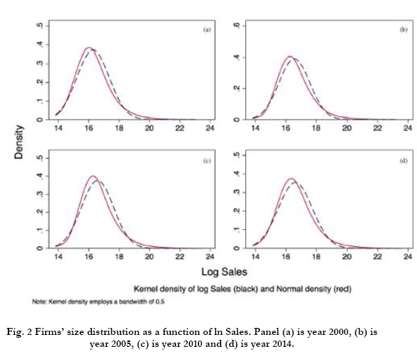
Following Segarra and Teruel (2012), we employ a Kernel density in order to estimate the empirical distribution of the logarithm of sales. A well-known benchmark distribution for the firms' size is the lognormal distribution, introduced by Gibrat in his seminal work (Gibrat, 1931). In the following, we test whether the empirical distribution of our sample can be reasonably described by the lognormal distribution. In Fig. 2, we plot the Kernel density as well as the lognormal density. As one can see, the empirical distributions are fat tailed, i.e. the upper tail of the distribution is heavier than the tail of lognormal.

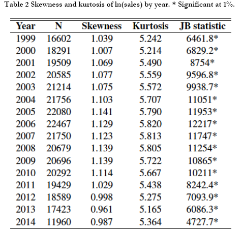
In order to test for Gaussianity of the distribution, we employed the Jarque-Bera test. The results are presented in Table 2, in which one can see that in the majority of the years under study there is a positive skewness and an excess of kurtosis. We can reject the null hypothesis of Normality in all the years at 1% significance level, and, therefore, we can conclude that the lognormal distribution is not a good description of the data. This finding is in line with other studies, such as Ganugi et al. (2005) and Reichstein and Jensen (2005). Note that under the lognormal distribution; we should not observe granular fluctuations, according to the theory developed by Gabaix (2011).

3.2. Power law distribution

Having ruled out that the whole empirical firms' size distribution follows a lognormal distribution, we focus our attention on the power law distribution, which is the family of distributions that has been used extensively in the literature, to describe the tail of the

firms' size distribution (see for instance: Axtell (2001); Bottazzi and Secchi (2003); Stanley et al. (1995)). In particular, we will consider the upper tail of the distribution of firms' sales, i.e. the distribution of the very large firms. The statistical characterisation of the empirical distribution is of crucial importance in determining the aggregate fluctuations. An exponential decay in the tail would, in fact, rule out large aggregate fluctuations, according to the Central Limit Theorem (CLT). Conversely, a heavy-tailed distribution can generate wide aggregate fluctuations.

In order to show graphically the heterogeneity of the empirical data, we employ the Complementary Cumulative Distribution Function (CCDF), i.e. the number of firms with a size greater than a given level S as a function of this level. The CCDF has been built arranging the firms of the sample according to their size, and assigning to each of them its rank.

From a first glance to Fig. 3, we can infer that there exists a high degree of heterogeneity among the volume of sales of the Spanish firms, comparing both, the size of largest firms with the average size of the whole sample and comparing the largest firms among them. For instance, taking the last year of the sample as a reference, one can see that Mercadona, the largest firm in this year, has roughly the double volume of sales than El Corte Inglés, the second largest firm. From a different perspective Mercadona has a size equal to the sum of the sales of the 3250 smallest firms of our sample. This anecdotal evidence, as well as the one shown in Figure 1, points to the existence of a large heterogeneity in the size of the Spanish firms.

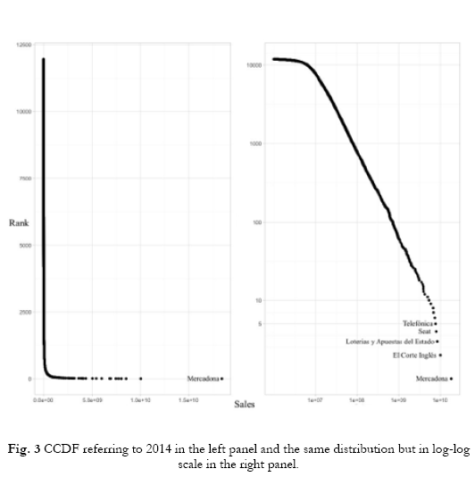
From a more quantitative point of view, it can be seen from right panel of Fig. 3 that the upper tail of the empirical distribution can be approximated by a straight line. In statistical terms, this means that the tail of the size distribution can be described using a power law distribution. The functional form of this family of distributions is:

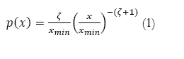
It is characterised by the tail index which represents the slope of the straight line describing the tail of the distribution. The parameter x_min represents a threshold above which the scaling relationship (1) holds (Alfarano and Lux, 2011).

The estimation of the index z allows us to quantify the degree of heterogeneity existing in the firms' size distribution. Maximum heterogeneity is reached when , which refers to the Zipf s law (Zipf, 1949). Higher values of the index suggest a lower degree of heterogeneity. According to the theory developed by Gabaix (2011), an index above 2, >= 2, indicates the absence of granular firms. The intuition behind this theoretical result relies upon the CTL. The aggregation of variables following a distribution with finite variance converges asymptotically to a Gaussian distribution. A tail index > 2 means that the variance of the size distribution is finite. Gabaix illustrates that this condition implies vanishing fluctuations at aggregate level. Conversely, the case 1 <= < 2 generates non-vanishing aggregate fluctuations even in the case of very large total number of firms. In the extreme case of = 1 the aggregate fluctuations decay proportionally to 1/ln (N).

The estimation is carried out following Clauset et al. (2009). We estimate the scaling parameter £ in our sample using Maximum Likelihood estimator, which is:

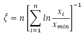
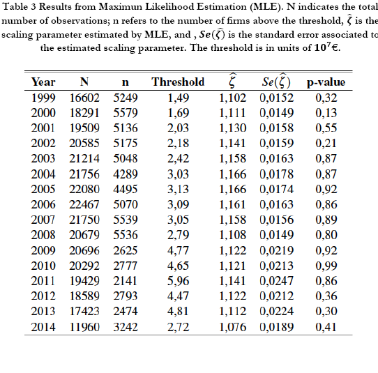
This estimator is also known as Hill estimator (Hill et al., 1975). Following Clauset et al. (2009), it has been tested the hypothesis that the firms size distribution is power law in its upper tail. The null hypothesis is the power law distribution and the alternative is the lognormal. As one can see in table 3, we cannot reject the null hypothesis for any year. Regarding the scaling parameter it is slightly above 1 for all periods.^§§§

Therefore, we can say that the distribution of large firms can be approximate by a power law distribution, reflecting a high degree of heterogeneity in the firms' size distribution. Based on these results, the level of heterogeneity should be sufficiently high to observe the phenomenon of granular fluctuations in the Spanish economy.

4. The model and its calibration

The main idea of the framework proposed by Gabaix (2011) is to connect the shocks affecting individual firms to the aggregate fluctuations of the whole economy. In order to connect the fluctuations at the firms' level to the aggregate fluctuations, it is necessary to characterise the firms' size distribution, or, at least, its upper tail. An additional ingredient to be consider is the way firms influence each other, for instance if they exhibit supply-chain type of interaction.

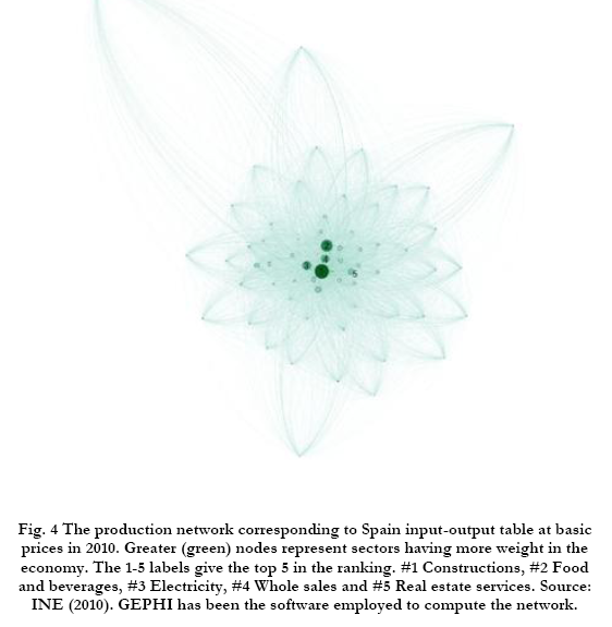
To compute the order of magnitude of the aggregate fluctuations, we will employ two different frameworks: the Island's model of Lucas**** and the full connected firms model of Hulten (1978). These two scenarios are obviously the extreme cases of a whole spectrum of possibilities. Fig. 4 shows the input-output network of the Spanish economy. It is clear that some of the sectors are more connected than others, showing that the Spanish economy is characterised by an intermediate configuration.††††

4.1. Independent Firms

The Islands' model assumes that all firms produce final goods and there is no link between them regarding the inputs used for production, namely, a company is not a supplier of any other firm. Under this assumption, the GDP growth of the whole economy can be expressed as:

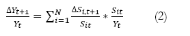
where is the annual change of GDP, and is the annual change in the volume of sales of firm i in year t. N indicates the number of independent firms (islands) that make up the economy. Equation (2) indicates that GDP growth is the sum of the growth of each firm, calculated as weighted by its relative size with respect to the whole economy.

If firms are independent, their growth rates are due to idiosyncratic shocks caused, for instance, by workers' strikes, change in management of the company, exogenous shocks in the firm's demand, etc.

Following Gabaix's approach and assuming that the sales growth rates have the same standard deviation , the relationship between GDP volatility and the volatility of firms can be expressed as:

where h is the square root of the Herfindahl index, a very typical measure of concentration in industrial organization. Here h represents a measure of dispersion of the distribution of firms's size, and it depends directly on the distribution of the relative size of the companies. This relationship implies that the volatility of the economic cycle is directly proportional to the volatility of growth rate of individual firms with a coefficient depending on the distribution of firms' size.

Assuming that all companies have a similar relative weight in the economy (h = 1/N), as it is implicitly assumed in conventional macroeconomic models, the volatility of GDP becomes:

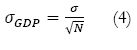
To check whether this holds true for the Spanish economy, the average of the standard deviation of firms' shocks in the sample has been calculated. Given that the number of companies in Spain is approximately three million, according to Eq. (4) fluctuations in the economic cycle would have a volatility of 0.019%. This result is not consistent with the empirical volatility of GDP, which is 4.36%‡‡‡‡. This simple calculation indicates the reason why conventional macroeconomic models, based on the paradigm of representative firm, consider aggregated and exogenous shocks as solely responsible for the business cycle fluctuations (for instance, adoption of new technologies by all companies, energy shocks, monetary shocks, political shocks, etc.).

Nevertheless, giving up to the assumption of homogeneity in companies' size and considering the empirical distribution of the heterogeneity of firms, the predicted GDP volatility would be 1.6%, which is the result of h_firm *, being h_firm = 4.81% the empirical value of the square root of the Herfindahl index. As can be seen, by taking into account the heterogeneity in the size of the companies empirically observed, the volatility predicted by Islands model is close to the empirical GDP volatility. The assumption of homogeneity among firms predicts a GDP volatility 230 times lower than the one observed empirically, while considering the empirical heterogeneity, the GDP volatility is just 2.7 times lower.

4.2. Fully connected firms

Despite the fact that the assumption of independent firms is very restrictive, it allows us to estimate quite precisely the order of magnitude of business cycle volatility, as long as the empirical heterogeneity among firms' size is considered. In the following we assume the existence of interaction among firms.

The theorem proposed by Hulten (1978) considers input-output interactions among firms, generalising the assumption of the Islands model based on independent firms. This theorem considers a configuration where all firms are suppliers of all the other firms, in a fully connected network. Like in the case of the Island's model, the fully connected network represents an extreme case. We use it as a benchmark model to approximate the empirical network. The Hulten's theorem states that Total Factor Productivity (TFP) growth can be decomposed in the sum of the idiosyncratic productivity shocks to individual firms weighted by the relative size of each firm in the economy:

where is the productivity shock of i in year t, and . Gabaix (2011) argues that GDP growth is directly proportional to the growth of TFP:

 

where . represents the use of production factors, such as capital and labor. The relation (6) is based on a common assumption considered in numerous growth models in macroeconomics, which states that the long-run growth is driven by technological progress.

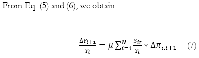
Calculating the standard deviation of GDP from Eq. (7), and assuming uncorrelated idiosyncratic productivity shocks, one finds:

In order to verify whether this Eq. (8) estimates a reasonable value to the observed GDP volatility, we use = 2.6, the value employed by Gabaix (2011), as well as the volatility of the proxy of productivity shocks proposed by Gabaix, which is , where E_it is the number of employees in firm i in the year t. From our sample of firms, the standard deviation of the empirical productivity growth is= 37% . So, using Eq. (8), we can estimate the GDP volatility, which turns out to be 4.6%, a value considerably close to the observed one (4.36%). This simple model of interactions among firms alongside the inclusion of a large heterogeneity in firm size enables us to predict the order of magnitude of macroeconomic fluctuations in GDP with astonishing precision.

 

5. Empirical Analysis

The calibration of the model, based on the Huten's theorem, shows a higher accuracy in predicting the GDP fluctuations with respect to the islands framework. We are, then, encouraged in using the Hulten's framework to test whether the Spanish economy exhibits granularity. Following the original methology of Gabaix (2011), we employ the following definition of "granular residual":

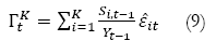
where is the estimated component of the factor productivity growth rate of a firm belonging to the K largest firms.^§§§§ This empirical granular residual is defined as:

The idiosyncratic productivity shocks are approximated by the relative productivity growth of firm i with respect t the average of the economy. Estimated idiosyncratic productivity shocks are the difference between the productivity growth rate, g_it , of firm i in year t, which is defined as: and g_t , which is an average of productivity growth. This average can be calculated taking into account the whole sample or limited to the sector to which the firm belongs (this procedure is called industry demeaning). The basic idea is that idiosyncratic fluctuations of a few large firms, K = 100, are sufficient to capture a significant fraction of economic cycle fluctuations. If N is the order of magnitude of one million businesses, K = 100 granular firms constitute only 0.01% of the entire sample. We have chosen the number of firms following Gabaix. We are aware that this choice is arbitrary. An effort in the development of the theory of granular macroeconomic fluctuations should go in the direction of endogenise such choice.

To quantify the explanatory power of the granular residual (G) on the aggregate fluctuations of GDP, a OLS regression is carried out. In particular, per capita GDP (GDPpc)^***** growth is regressed against the granular residual:

where two lags have been included.

If the economy is granular, an extremely small number of companies, such as the 100 largest firms, should account for a significant fraction of GDP fluctuations.

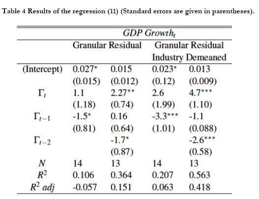
The results obtained from the estimation of equation (11) are shown in Table 4. As it can be seen, when the second lag is included the explanatory power of the granular residual improves in both cases, with and without industry demeaning. The former is able to explain 15% of the GDP growth variability, whereas the latter captures up to 42% of the variability. This means that the granular residual by itself (i.e., the measure that reflects the idiosyncratic shocks of the 100 largest firms, weighted by their relative size in the economy) is able to explain more than half of the per capita GDP variability during the time period studied.

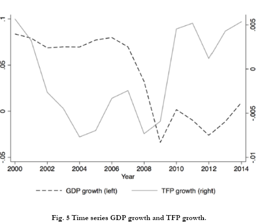
Interestingly, some of the regression coefficients turn out to be significant and similar in magnitude to the ones computed by Gabaix for the US economy, however, they have a different sign. The Spanish economy exhibits an inverse relationship between GDP growth and granular companies' fluctuations. One possible explanation of the discrepancy of our results with respect to the Gabaix findings is that Spain is characterised since 1990 by having showing a decline in TFP. Fig. 5 shows the time series of GDP growth and TFP growth. During the period of time between 1999 and 2014 the correlation between GDP growth and TFP growth is -0.3. The negative correlation can be partially due to the relatively high weight of low productivity sectors. As it can be seen in the input-output network (Fig. 4), sectors with higher weight in the Spanish economy are the ones with low productivity, such as real estate services and constructions.

This work indicates that the granular nature seems to be relevant in the description of the Spanish business cycle. It should be noted, however, that the work has some limitations due to the short period of time considered. More empirical analysis and the development of the theory of granular macroeconomics are needed for firmer conclusions.

 

6. Conclusion

The empirical evidence shows that the Spanish economy exhibits a granular behaviour, indicating that a small number of companies have a significant impact on business cycle fluctuations. This result is the consequence of the high degree of heterogeneity among firms, which makes that, in the aggregate, idiosyncratic shocks of large firms do not average out.

The granular residual accounts for approximately half of the variability in GDP fluctuations of the Spanish Economy. Our results are in line with the (yet few) empirical contributions exiting in the literature supporting the reliability of the granular hypothesis.

As a future research we are currently working on endogenise the selection of the number of granular firms, beyond the simple exogenous rule when fixing that number.

 

Notas

*** The number of firms in 2015 was 3.168.878, according to Directorio Central de Empresas [Instituto Nacional de Estadística (INE)].

††† The acronym stands for Standard Industrial Classification, which is a four-digit code that classifies firms according to their businesses.

The estimations of the Table 2 has been carried out using the R package poweRlaw (Gillespie, 2014).

§§§ The reader should note that we do not pretend to perform an exhaustive empirical analysis on the scale free nature of the tail distribution of firm size. We have employed a widespread technique whose results coincide with other economies, so that “the Spanish case” is in line with the existing literature.

**** The model was formulated in a series of papers, see: Lucas (1972, 1973, 1975).

†††† Acemoglu et al. (2012) take the input-output network to explain how shocks propagate among sectors. They claim that, depending on the network structure, idiosyncratic shocks cannot be localised in a sector, but spread across the economy, affecting the output of other sectors.

‡‡‡‡ GDP data was taken from INE (2016a).

§§§§ Following Gabaix, to avoid possible distortions arising from excessively high productivity shocks, a winsorising is employed. Consisting in:

***** GDP per capita was taken from INE (2016b).

 

References

Acemoglu, D., Carvalho, V. M., Ozdaglar, A., & Tahbaz-Salehi, A. (2012). The network origins of aggregate fluctuations. Econometrica, 80(5):1977-2016.        [ Links ]

Alfarano, S. & Lux, T. (2011). Extreme Value Theory as a Theoretical Background for Power Law Behavior. Working Papers 2011/02, Economics Department, Universitat Jaume I, Castellón (Spain).        [ Links ]

Axtell, R. L. (2001). Zipf distribution of us firm sizes. Science, 293(5536):1818-1820.        [ Links ]

Blank, S., Buch, C. M., & Neugebauer, K. (2009). Shocks at large banks and banking sector distress: The banking granular residual. Journal of Financial Stability, 5(4):353-373.        [ Links ]

Bottazzi, G. & Secchi, A. (2003). Common properties and sectoral specificities in the dynamics of us manufacturing companies. Review of Industrial Organization, 23(3-4):217-232.        [ Links ]

Carvalho, V. M. & Grassi, B. (2015). Large firm dynamics and the business cycle. Technical report, CEPR Discussion Paper No. DP10587.        [ Links ]

Clauset, A., Shalizi, C. R., & Newman, M. E. (2009). Power-law distributions in empirical data. SIAM review, 51(4):661—703.        [ Links ]

Del Rosal, I. (2013). The granular hypothesis in eu country exports. Economics Letters, 120(3):433^36.        [ Links ]

Di Giovanni, J. & Levchenko, A. A. (2012). Country size, international trade, and aggregate fluctuations in granular economies. Journal of Political Economy, 120(6):1083-1132.        [ Links ]

Fernandez-Villaverde, J., Garicano, L., & Santos, T. (2013). Political credit cycles: the case of the eurozone. The Journal of Economic Perspectives, 27(3):145-166.        [ Links ]

Gabaix, X. (2011). The granular origins of aggregate fluctuations. Econometrica, 79:733-772.        [ Links ]

Ganugi, P., Grossi, L., & Gozzi, G. (2005). Testing gibrat's law in italian macro-regions: analysis on a panel of mechanical companies. Statistical Methods and Applications, 14(1):101—126.        [ Links ]

Gibrat, R. (1931). Les inégalités économiques. Recueil Sirey.        [ Links ]

Gillespie, C. S. (2014). Fitting heavy tailed distributions: the powerlaw package. arXiv preprint arXiv: 1407.3492.        [ Links ]

Hill, B. M. et al. (1975). A simple general approach to inference about the tail of a distribution. The annals of statistics, 3(5):1163—1174.        [ Links ]

Hulten, C. R. (1978). Growth accounting with intermediate inputs. The Review of Economic Studies, 45(3):511-518.        [ Links ]

INE (2010). Input-output framework. (accessed on 31 october 2016). http://www.ine.es/jaxi/menu.do?type=pcaxis&path=%2Ft35%2Fp008&file=inebase&L=1.        [ Links ]

INE (2016a). Producto interior bruto (pib). (accessed on 31 october 2016).http://www.ine. es/prensa/pib_tabla_cne.htm.        [ Links ]

INE (2016b). Producto interior bruto (pib) per cápita a precios corrientes by país and periodo. (accessed on 31 october 2016). http://www.ine.es/jaxi/Tabla.htm?path⁼/t42/p05/l0/&file=05001.px&L=0.        [ Links ]

Kydland, F. E. & Prescott, E. C. (1982). Time to build and aggregate fluctuations. Econométrica: Journal of the Econometric Society, pages 1345-1370.        [ Links ]

Lucas, R. E. (1972). Expectations and the neutrality of money. Journal of economic theory, 4(2):103-124.        [ Links ]

Lucas, R. E. (1973). Some international evidence on output-inflation tradeoffs. The American Economic Review, 63(3):326—334.        [ Links ]

Lucas, R. E. (1975). An equilibrium model of the business cycle. The Journal of Political Economy, pages 1113—1144.        [ Links ]

Lucas, R. E. (1977). Understanding business cycles. In Carnegie-Rochester conference series on public policy, volume 5, pages 7—29. North-Holland.        [ Links ]

Reichstein, T. & Jensen, M. B. (2005). Firm size and firm growth rate distributions—the case of denmark. Industrial and Corporate Change, 14(6):1145-1166.        [ Links ]

Segarra, A. & Teruel, M. (2012). An appraisal of firm size distribution: Does sample size matter? Journal of Economic Behavior & Organization, 82(1):314-328.        [ Links ]

Stanley, M. H., Buldyrev, S. V., Havlin, S., Mantegna, R. N., Salinger, M. A., & Stanley, H. E. (1995). Zipf plots and the size distribution of firms. Economics letters, 49(4):453^157.        [ Links ]

Wagner, J. (2012). The german manufacturing sector is a granular economy. Applied Economics Letters, 19(17):1663—1665.        [ Links ]

Zipf, G. K. (1949). Human behavior and the principle of least effort. Technical report, addison-wesley press.        [ Links ]