


 Inglés (pdf)
 Articulo en XML
 Referencias del artículo
 Enviar articulo por email
 Citado por SciELO
  Similares en
SciELO
Similares en
SciELO 
 Permalink
1. Introduction
During the last years, some Bolivian authors have highlighted low and decreasing returns to education in Bolivia using the traditional 'Mincerian approach' developed first by Mincer (1974) with the use of information of annual household survey conducted by National Statistics Office (INE due its acronym in Spanish).
For instance, Villarroel and Hernani (2011) found that returns to education have decreased during the first decade of this century from 10% to around 5%. They do not hypothesize about the causes of this trend, although they discard education supply roots. Later and in a broad study focused on the roots of the declining poverty and inequality, Vargas and Garriga (2015) also found this pattern using both Mincer approach and with a correction of the omission bias using the approach proposed by Heckman (1979). Moreover, they include a set of controls that helps to isolate education returns.
Using more actual data from the same source, Andersen (2016) also found a similar drop from 11% in 1999 to nearly 4% in 2014. She highlighted the fact that returns were statistically above 0% even for the low return sector (transportation). Besides, she first suggested that linearity in the Mincer equation was absent in 2014. More interestingly, she provided some possible reasons for this decline. On the supply side, she attributed it to the expansion of skilled people mainly in the last years, while on the demand side she considered increased demand of unskilled people given the boom in some commodities' markets.
In what follows I will analyze the returns to education using both the standard 2015 household survey and the Demand for Skills Survey carried by the IADB in similar months. I found that even the standard specification is linear in the (transformed) variables, returns could vary according to the particular year of schooling and some milestones related to the end of specifics education stages. I also use the theoretical framework developed by Bobba et al. (2018) to set the econometric estimation of a multinomial logit model with four choices to estimate earnings equation for self-employed, informal workers and formal workers.
In that sense, I found evidence supporting a Mincer equation with non-linearities in the Bolivian case as was suggested for the US case by Card and Lemieux (2001) and Heckman et al. (2006).
The paper is organized as follows. After this introduction, I will discuss the data used in this analysis focusing on the characteristics related to the estimation. Then I will present some Mincerian estimates to discuss the underlying non-linearity Finally, I will try to explain the results focusing on the role of informality and segmented labor markets.
2. Data and methodology
Most of the econometric analysis carried in this paper rest on the the 2015 annual household survey (best known as 'Encuesta de Hogares 2015' in Spanish) which is a yearly assessment carried by INE2. I will discusse its main characteristics, specially the ones related to the econometric estimation.
Regarding education, the survey includes years of education and the highest level attained. But one of the measurement problems is that Bolivia has experienced at least three partial reforms in educational levels in the last 20 years. So definition of primary and secondary education vary Moreover, there is not a technical analysis of the differences in the syllabus of every reform.
Concerning occupation, it is worth noting that INE considers a person employed if he/she worked at least one hour in the week before the survey It also covers people aged 7 years and older given the extent of child work, mainly in rural areas.
For our purposes, it is important to mention that omission bias could be avoided directly from the survey because an unemployed person is asked for reasons not to look for a job, including unfruitful previous search, perceived and efective discouragement and expectations of better offers.
It also includes questions on weekly days and daily hours in the job. Unfortunately, it does not have a question on total years of experience, just current job experience. Because of a large extent of informal sector and self-employment, it has a lot of questions on primary and secondary occupation.
The vast size of informal sector, around 60% according to Velasco (2015), represents a challenge for a Mincerian estimation. In fact, this kind of estimation is used as wage equation, while in the Bolivian case it involves both wage and 'petty entrepreneurs' income, as it is noted by Villarroel et al. (2012).
In fact, 2015 survey includes 14,630 observations on labor income. But there were just 6,882 employees in the strictus sensus, because the remaining cases belong to entrepreneurs, self-employed people or even apprentices. And if we consider those who contribute to the pension system there are just 2,802 observations.
Thus, the results of a Mincerian equation of the whole sample must be taken with caution, because they do not represent a wage equation, but a reduced-form earnings equation.
To avoid these risks, I add more control variables to the main equation in order to isolate the effect of education on 'labor' income, following the approach of Vargas and Garriga (2015).
Additionally, I employed data from a survey carried out on skills. In 2012 the Inter-American Development Bank released a report titled 'Disconnected: Skills, Education, and Employment in Latin America' in Bassi et al. (2012). The main concern of this volume was to show the disconnection between the labor market and the educational and training system in the region.
One of the chapters of that book was devoted to understand the concernings of the employers regarding skills and general and specific abilities of the workers. So, the IADB conducted a survey in Argentina, Brazil and Chile from around 1,200 firms.
The survey was a 'Demand for Skills Survey' (DSS), a standard instrument for a better understanding of labor demand, mainly regarding some characteristics considered as useful for firms in order to have higher productivity. Besides, the IADB could estimate a skill gap between supply and demand in the labor market.
Five years later, the Bolivian government agreed to carry out this survey in the main three cities of the country (La Paz, Cochabamba and Santa Cruz). A general discussion about the results can be found in Urquidi (2015).
Bolivian DSS was conducted between January and April of 2015 to 1,831 firms, most of them SME, while a quarter of the sample was devoted to the medium and big firms. It was conducted following the guidelines of the IADB to have comparable results with the 2012 report. It was in charge of the Information and Statistic Collection Center at the Private University of Bolivia (CEGIE).
The questionnaire comprises around 90 questions, including a) detailed list of main jobs specifying gender, age, experience and wage for each item; b) effects of labor regulations; c) skills assessment of the three main non-administrative jobs; and d) training.
Given the length of the survey, just 460 medium and big firms answered the section devoted to the skills assessment. Thus, the results are biased to them. However, given that twenty jobs inside the firm are assessed we have potential answers for more than 4,000 employees.
Regarding the methodology, I begin with some basic explorations on the nature of the relationship among schooling and earnings, showing some signs of a non-linear association.
Then I estimate a reduced form of earnings equation controling for other factors as ethnicity, gender, urbanization, among others in two forms: simple OLS technique and omision bias corrected regression.
After that, I employ a segmented labor approach to understad in which segment (unemployed, self-employed, informarl worker, or formal) this non-linear relationship is more relevant.
Finally, I use the IADB data corrected with a matching algorithm to estimate this earnings equation with information from firms rather than workers. This procedure gives us a detailed view of the main determinants of earnings and the effect of informality3.
3. A simple and preliminary exploration of effects of education on earnings
Before the estimation, I made an analysis of years of experience according to the highest educational level attained by individuals. To simplify the analysis and avoid the wide range of earnings, I use the median income for each year of experience.
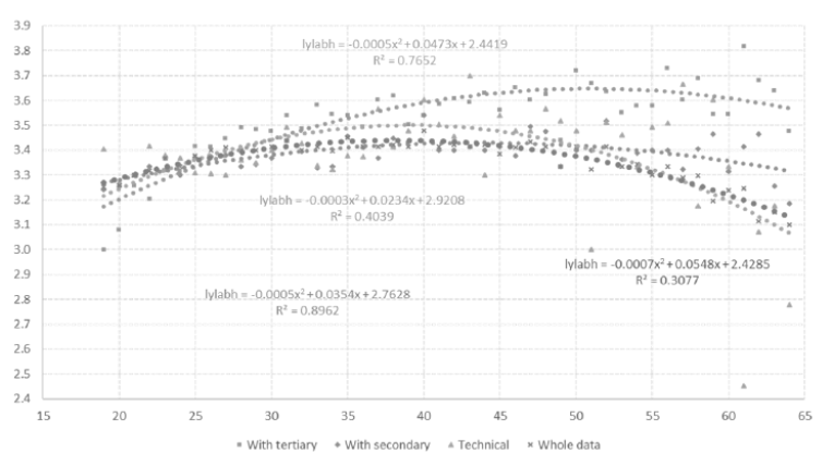
As Figure 1 shows, there is a similar pattern among median income and experience for each educational level, a non-linear shape that is clearer for the whole data. Then the quadratic form of experience seems appropriate for this set of data.
Following a similar approach, I calculated some statistics of (log) hourly earnings according to educational levels to find out whether different returns to education emerge previous to regression analysis (Table 1). It seems obvious that a higher educational level is associated to a higher income although high variability of earnings for each level do not allow us to reject the alternate hypothesis of different mean earnings between reported levels.
Source: Own calculations based on Encuesta de Hogares 2015.
Figure 1: Median income for each year of experience for people with secondary, tertiary, technical education and whole data
Table 1 Log of hourly earnings by educational level
Source: Own calculations based on Encuesta de Hogares 2015.
Letting aside this detail, it could be inferred that primary education provides an annual average return of 12% compared to no schooling. Following similar criterion, secondary education adds an annual mean return of 8.5%. Finally tertiary education represents an average return of 10%. It must be noted that this analysis does not consider the experience factor or other relevant control variables.
The next step is to proceed with the estimation of a Mincerian earning equation. In its simple form, Mincer equation is a relationship between hourly earnings, years of education and a quadratic expression related to experience. The result of the simplest case is the following:4
So, this simplest form suggests an annual mean return of schooling of 7.8%, above other estimates, although the exclusion of other control variables clearly gives biased estimates of this parameter. In the case of experience, this initial estimation suggests a concave function of years of experience. Earnings increase until they reach a maximum at 27 years of experience independent of schooling years.
Also, I will estimate as a preliminary exercise a polynomial version of the previous equation to look for non-linearity on returns of education. As I will explain in the next section, I am using a 4th degree polynomial:
To obtain the average return of education for the whole sample, consider a vector
Then the average return is given by equation (3):

Using this equation, the weighted average return of education is 7.9%, which does not differ from the linear form. However, we will see later that it implies different rates for each educational level.
4. Standard single equation estimation of earnings equations
To isolate with more accuracy the effect of education, I have regressed the hourly earnings according to this specification:
Ergo, I have added many other variables that could affect earnings levels with results shown in Table 2. Most of them are included as a 'slope effect' or as a dummy variable multiplied by schooling, rather than just a dichotomous variable for intercept effect. I will explain the most relevant regarding the purpose of the estimation.
One key variable is informality. In fact, formal/informal categories were defined as follows: formal with long-term social security (pension system) and short-term (medical insurance); two categories of semi-formal with or long-term or short-term social security; and informal to those who do not have neither long nor short term social security.
To avoid omission bias I started with the inclusion of a large set of variables given more than enough available degrees of freedom. Then I have left just the significant variables. Using the previous approach, I calculated that the average return to education is around 2%.
Table 2 Estimate of linear multiple control Mincer equation
Source: Own calculations based on Encuesta de Hogares 2015.
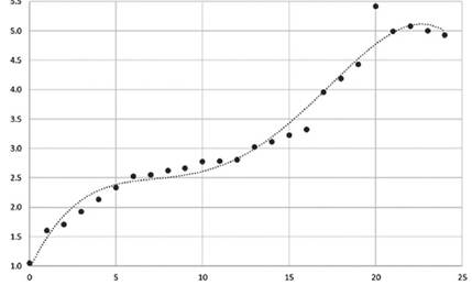
To analyze with more detail the effect of education, I removed the effects of control variables except for education. Thus, I computed the conditional income. Then I calculated the mean for each year of education. A clear pattern of non-linearity also arose showing different rates of return for each year, shown in Figure 2.
Source: Own calculations based on Encuesta de Hogares 2015.
Figure 2: Conditional mean income and years of education
Then I included this polynomial form in the whole equation also corrected by the weights provided by INE to extrapolate results to whole population, the results are reported in Table 3. These results are also consistent with an average return of 2.3%, slightly above regarding the linear effect of education reported in Table 2.
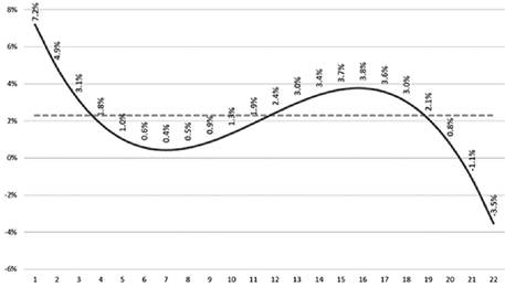
Nevertheless, the pattern differs according to each year of education. As it is showed in Figure 3, year 1 represents a marginal return of 7.2%, probably explained by the effects of writing and reading skills.
Then the marginal return decreases until the first year of secondary education, where there is an inflection point. So, returns to education gradually increase reaching their local maximal around the end of tertiary education. Finally, graduate education is just profitable on average for short courses. Anyway, cumulative returns differ in statistical terms just for tertiary education given the variation within a year, even controlling for other variables.
Table 3 Estimate of multiple control non-linear Mincer equation
Source: Own calculations based on Encuesta de Hogares 2015.
Source: Own calculations based on Encuesta de Hogares 2015.
Figure 3: Average and marginal return to education for each year of education
Other remarkable results related to schooling returns are:
For each year of education, a formal worker has an additional 2% of return, a semi-formal 1% and an informal -1%.
For each year of education, commerce represents 2% less of return, industry 1% less and mining 3% more than the average.
Returns to education are lower than the national average in Chuquisaca (1%), Oruro (1%) and Potosí (2%) for each year of education.
Migrants to Santa Cruz have 2% more of returns for every year of education.
Finally, I corrected the estimation with the ‘selection bias' according to Heckman (1979). I employed a logit model of selection with gender, marital status, ethnicity, and the position of the worker in the family. Then the estimation included the inverse Mills ratio to deliver unbiased estimates, shown in Table 4. Compared with the OLS estimates, it implies an average return of2.8%, mildly above the linear and non-linear effects of education reported previously
Table 4 Sample selection corrected non-linear Mincer equation
Source: Own calculations based on Encuesta de Hogares 2015.
Besides, it points out that unobservable characteristics of workers imply higher probability of selection for employment if they are highly skilled, according to the interpretation suggested in Narayanan (2015).
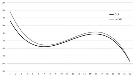
The pattern of marginal effect of an additional year of schooling on earnings is like the non-linear estimate but with higher marginal effects at the basic levels of education, as shown in Figure 4.
Source: Own calculations based on Encuesta de Hogares 2015.
Figure 4: Marginal return to education for each year of education
To summarize this section, if we analyze returns to education with the standard approach of a single equation estimation, a non-linear approach seems better than the linear one controlling by other factors. The temporal pattern of marginal returns points at least two peaks: one associated to basic reading and writing skill and other to complete undergraduate studies. In the next section we will explore a more suitable approach for segmented markets.
5. A segmented labor market approach
Even the insights of the previous section and a more elaborated version with the sample selection technique could be misleading because Bolivian labor market is not similar to the ones of other developed countries.
In fact, and following Bobba et al. (2018), we can consider that the Bolivian labor market has four segments:
Then a broader approach must include both the matching and the search processes involved in this estimation procedure.
Even the cited authors employ the Simulated Method of Moments to the complete model estimation, I follow their logic to estimate a multi equation model in two stages. So, I employed the multinomial or categorical response model described in a general approach in Cramer (2003) and with more details in Glewwe (1992) and implemented for a similar case in Gunther and Launov (2006), I estimated this model for these four categories (formal, informal, self-employed and unemployed) taking the last one as the baseline model. Results are shown in Table 5.
With these estimates, I calculated three earnings equations whose results are available in Table 6. Selection bias is only present in the informal earnings equation, where the implied negative relationship (i.e, a positive sign of the correction term) could mean that a higher (lower) productive worker with a higher (lower) chance to be selected in this market has a lower (higher) wage. So, we have a plausible explanation of the low returns due an adverse selection phenomenon in informal market due to information asymmetry as pointed out by Narayanan (2015).
I must mention that the weighted average return of schooling is lower in the self-employed group (6.6%) than informal employees (10.1%) and formal ones (14.9%).
6. Returns according to labor demand from firms
Previous earnings estimates come from different kinds of households. On the other hand, IADB survey is focused in formal firms.
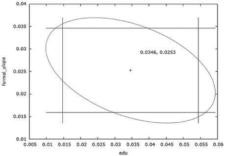
To address the compatibility between these databases I calculated the Mahalanobis distance between them. The results show that taking the whole INE database, IADB is more concentrated around the upper income and education segments. If we focus only on formal sector, there is a clear intersection among them as it is suggested in Figure 5.
To assess this feature, I employed the nearest neighbor matching algorithm based on the Mahalanobis distance taking into account some set of information as age, education, region and gender, leaving aside the income, following the guidelines of Caliendo and Kopeinig (2008). After picking the nearest neighbor, I compared the densities of (log) incomes and carried a Kruskal Wallis test, not rejecting the hypothesis that they come from a similar distribution (Figure 6).
Consequently, I used the micro-data of this survey to try to consider the effects of schooling and informality of labor demand in the Bolivian case but with primary data from the firms, rather than the usual approach of using the Bolivian annual household survey to have an earnings equation.
Table 6 Segmented labor market earnings equations
Source: Own calculations based on Encuesta de Hogares 2015.
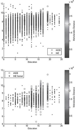
Source: Own calculations based on INE and IADB surveys.
Figure 5: Comparison of IADB and INE surveys in the log(income) and education space
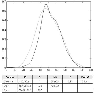
Source: Own calculations based on INE and IADB surveys.
Figure 6: Densities of IADB and INE matched observations and Kruskal Wallis test
Then I used the Heckman approach to estimate both linear and non-linear equations with IADB information (Table 7). Two clear patterns arose: i) the statistical no significance of the factor associated to the selection bias, and ii) a nonlinear shape of the returns to schooling in the formal sector5. Besides, weighted average is around 12%, close to the mean return of 15% of the multi-equation approach of the previous section.
To assess the gap between formal and informal workers, I must mention that the matching process described above delivered 72 cases (near 8%) of matched pairs between formal and informal workers. A simple test about the average difference delivered that on average, a formal worker with similar characteristics of an informal has an income 41% higher than the last one.
Table 7 Selection sample correct estimation of formal labor demand
Source: Own calculations based on IADB 2015.
To refine this result, I ran a regression with a slope effect with the following results:
As it is implied in Figure 7, the average return gap among formal and informal earnings varies between 2% and 4% for every additional year of schooling. This is coherent with this gap of near 40% mentioned previously.
7. Concluding remarks
I showed that the puzzle of low average returns could be explained by non-linearity in the earnings equation. Specifically, it could be noted that acquiring a college degree or a university degree could give higher income on average.
But with a more careful analysis, I hypothesized that this pattern is due to a segmented labor market where informal and self-employed workers have lower returns than formal ones. Even more, people with similar age, education, gender, and sector have lower returns on schooling.
Even though this finding seems intuitive given the nature of informal markets, further research is needed. The simplest way is to run a non-parametric regression to capture better this nonlinear relationship, while an advanced one is to find the roots behind this earnings distribution and its relationship with schooling is found in Bobba et al. (2018)).
They built an economic model with segmented markets, where the optimal schooling decision was made before entering the labor market. So, they discuss the distortions in that deliver different returns.
Future research could estimate the model for the Bolivian economy, as they for the Mexican economy. This would give more insights on the issue of why education could be wasted years for a huge part of Bolivian population.

