1. Introduction

Historically, the agricultural sector in Paraguay has played a key role in economic development and contributed significantly to economic growth (^{World Bank, 1995}). Approximately 65 percent of households in rural areas rely on some sort of agriculture-related income (e.g., working on their own land or as employees in agriculture-related activities). Even in urban areas this share is about 17 percent. During the first decade of the 2000s, Paraguay's extreme poverty has been stubbornly stable at around 18 percent, despite the sizable growth in average individuals' incomes and high rates of economic growth. Part of the explanation for this stylized fact is related to the increase in food prices. Between 2005 and 2007, basic food basket prices outpaced the overall inflation rate becoming more expensive and despite the real income of the poorest quintile was growing it was not enough to compensate for the price increase. This phenomenon reveals how fluctuations in food prices can affect household welfare through different channels in countries where a large share of households is both consumers and producers of basic food. Moreover, those effects on welfare are far from being obvious (i.e., higher prices harm households on the consumption side while they can benefit them on the production side through higher incomes).

Since developing economies, and fundamentally those dependent on agriculture, are permanently exposed to food price fluctuations the objective of this paper is to simulate the welfare effects of a potential hike in food prices in Paraguay. Following the traditional agricultural model, originally proposed by ^{Singh et al. (1986)}, we simulate three different effects of higher prices on households' welfare: (i) the expenditure effect, as consumers face more expensive prices; (ii) the income effect, as profits for farm holders or wages for employees in agricultural activities increase; and (iii) a government policy response, simulated as an increase in the amount of the cash transfer to current beneficiaries of the existing social program Tekoporã¹. We simulate an increase in food prices similar to the one observed between September 2010 and August 2011, when annual food inflation was 17 percent while overall inflation was around 9 percent (5.4 percent if we exclude food items). We combine three sources of information. First, as baseline data, we use the 2011-2012 Income and Expenditure Survey (Encuesta de ingresos y gastos y condiciones de vida - EIG-CV henceforth) to characterize households in terms of incomes and expenditures (i.e., consumption patterns). Second, we simulate on the EIG-CV a food price hike using monthly price data collected in Greater Asunción by the Central Bank of Paraguay Here we consider heterogeneous price movements across 9 sub-categories of food items. Third, we simulate on EIG-CV the potential effect of a policy response by using the 2015 Permanent Household Survey (Encuesta permanente de hogares -EPH henceforth)².

Our main results suggest that the expenditure effect is negative and, as expected, regressive for all households, but larger in rural than urban areas. The income effect, largely dominated by greater profits of those self-employed, is positive and progressive in rural areas while negligibly in urban areas³. Therefore, we find that the overall impact of an unexpected increase in food prices in Paraguay has a very flat U-shaped curve effect (i.e., those households at the extremes of the welfare distribution are less affected), similar to what ^{Ferreira et al. (2013)} found for Brazil, with an increase in extreme and moderate poverty Government policy response produces an ambiguous effect on vulnerable households. For instance, quadrupling the amount of existing monthly cash transfer would compensate the loss due to higher food prices but not everywhere. There would be fewer households in extreme poverty in rural areas while an extra effort would be necessary to help those in urban ones. On the contrary, the moderate poverty rate would be two points less than the pre-shock level after the transfer’s relief.

We believe our contribution is twofold. First, we contribute by providing evidence on the effects of a hypothetical price increase disentangling the impacts on consumers and producers, as well as in rural and urban areas. We focus on a country that has not been studied yet and where the agricultural sector plays a major role in the national economy Second, we contribute by estimating a sub-component of the income effect (i.e., the profit effect ) that was not considered in the existing literature (at least for Latin American countries). This contribution is relevant since the profit effect explains a substantial part of the final results. With this contribution, we provide additional evidence to a relatively scarce but growing literature. Existing studies support that the distributional effects of staple prices differ depending on the share of net-consumers and producers along with the income distribution. ^{Deaton (1989)} analyzed the distributional effects of price changes on households’ real income in Thailand, considering their role as both consumers and producers. ^{Benjamin and Deaton (1993)} and ^{Ravallion and van de Walle (1991)}, provided a similar analysis for price changes in Ivory Cost and Indonesia, respectively. ^{Ravallion (1990)} incorporated labor market responses to changes in food prices in rural Bangladesh into the estimation of welfare effects. ^{Ivanic and Martin (2008)}, made arguably one of the first attempts to do a cross-country analysis. Using households survey data for ten low-income countries they found an overall poverty- increasing impact of higher food prices because, in their sample, poor individuals are majorly net-consumers of food (both in urban and rural areas)⁴. Similarly, ^{Robles and Torero (2010)} analyzed four Latin American countries finding that a hike in food prices affects those food- importer countries and poor households in urban and semi-urban areas. Finally, there are two interesting case studies of a single country in Latin America. ^{Ferreira et al. (2013)} studied the impact of food prices on welfare in Brazil in 2008, considering the income effect of prices (only) on wages. ^{Attanasio et al. (2013)} estimated the effects of food prices in Mexico accounting for substitution effects on the demand side (but did not include income effects on the producer side)⁵.

The paper is structured as follows. Section 2 introduces several stylized facts of the Paraguayan economy. Section 3 presents data on household surveys and prices used in the empirical analysis. Given that prices are regularly observed only in urban areas; Section 4 discusses whether these prices are indeed a good approximation of prices faced in rural areas. Section 5 describes the analytical framework to assess the effect of a price increase on households' welfare and provides a brief literature review. Section 6 presents the simulation and main results. Section 7 analyzes the potential effects of different policy responses. Finally, concluding remarks are presented in Section 8.

2. Context

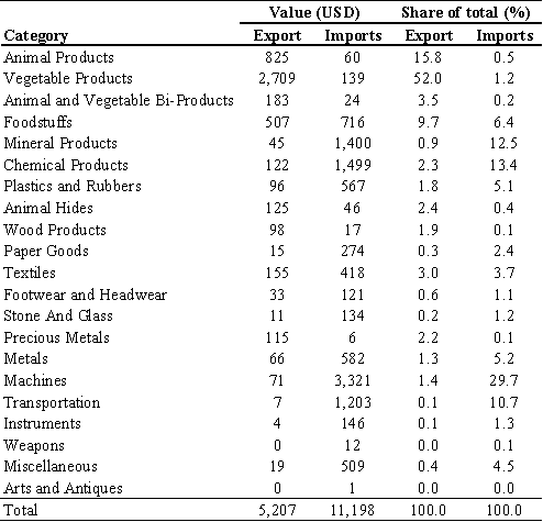
Paraguay is a small country with approximately 8 million inhabitants, located in South America. Its economy mostly depends on agriculture which in turn makes it more volatile (^{World Bank, 2014b}). Growth in agriculture has explained over 80 percent of the variation of real GDP growth since the early 90s. In the period 2003/13, real per capita GDP grew by 33 percent but experienced a major dip during the 2009 drought and global financial crisis when it fell by 5.2 percent with respect to the previous year. Yet, the record growth of 11.2 percent in 2010, driven by a 50 percent growth in agriculture, more than compensated that major dip. In 2014, the agriculture sector represented 25 percent of total GDP and 40 percent of national exports (World Bank, ^2014a and ^b). The country is a net exporter of agricultural and livestock products, and a net importer of foodstuffs such as prepared foods, beverages, etc. (Table 1).

Table 1 Exports and Imports by sub-category for Paraguay, year 2012 

Source: ^{Simoes & Hidalgo (2011)}; ^{Hausmann et al. (2011)}.

Since 2005, the prices of many food items have risen considerably (Figure 1). In the middle of 2008, the international food price index was 80 percent higher than in 2005. Then, it dropped massively by the end of the year. A second and equally sizable hike was observed in early 2011. “[P]rice increases of this magnitude for basic foodstuffs, over a relatively short period, led to widespread concern about possible impacts on hunger and deprivation” (^{Ferreira et al., 2013}). In this sense, higher food prices negatively affect the purchasing power of households, bringing them closer to situations of greater income vulnerability and poverty⁶. However, if household income is linked to activities associated with food sales at higher prices, they may experience an increase in their purchasing power, moving away from situations of greater vulnerability Since agriculture is one of those activities that are highly dependent on food prices, households whose income is associated with this sector could benefit from higher prices in the form of higher benefits for farm holders or higher salaries for employees.

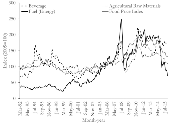
Source: International Monetary Fund.

Figure 1: Monthly evolution of commodity prices, 1992-2015 (2005=100, in terms of U.S. dollars) 

Given that the Paraguayan economy mostly depends on agriculture, the effects on the income side are relevant in rural areas. In countries such as Paraguay, which are large producers and exporters of foodstuff, a price hike leads to both a loss for net buyers of food items (mostly, urban households) and to a gain for net sellers (mostly, rural households)⁷. Overall, how higher food prices affect incomes and poverty in an agriculture-dependent country is not obvious. In this context, inquiring on these effects for Paraguay is very relevant. Most of all since two-thirds of the extreme poor people live in rural areas.

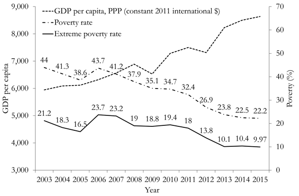
As prices fluctuated, between 2003 and 2013 Paraguay performed substantially well in terms of poverty reduction, showing sizable reductions in moderate and extreme poverty. This was the result of a period with significant economic growth combined with a reduction in inequality. A significant share of these improvements in welfare were only experienced after 2011. Before 2011, extreme poverty remained stable despite per capita GDP increased by 22 percent. Between 2011 and 2013 extreme poverty almost halved (Figure 2). A key factor behind the evolution of poverty rates in this decade was related to changes in food prices (^{World Bank, 2015}). While both growth and inequality reduction (redistribution) were contributing to a significant increase in the income of the poor during the period 2003-2011, food prices were rising at a higher rate than the general price index, mitigating to a significant extent the reduction in extreme poverty⁸. In contrast, these three forces (growth, inequality reduction and changes in food prices) worked in the same direction since 2011 (Figure 3). The sizable income growth among the less well-off and especially in rural areas was a strong factor behind the recent improvement in poverty reduction. In both periods, higher labor incomes derived from higher earnings (and higher number of earners) have been the driving force of this reduction. Since 2013, non-labor incomes such as public transfers started to play a significant role (^{World Bank, 2015}).

Source: DGEEC, WDI and own calculations.

Figure 2: GDP and poverty rates evolution 

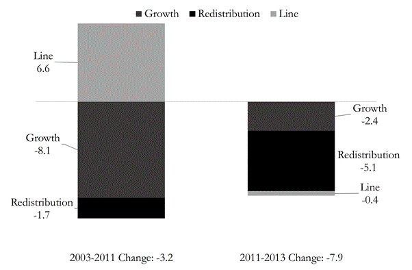
Source: DGEEC and own calculations.

Notes: Shapley decomposition is estimated, see ^{Shorrocks (2013)} for a detailed explanation on the methodology. Each bar presents the contribution of growth, income redistribution and change in food prices (line) to the change in poverty during 2003/11 and 201113, respectively. Bars below (above) the horizontal line indicate a positive (negative) contribution of each factor to poverty reduction.

Figure 3: Decomposition of changes in extreme poverty  

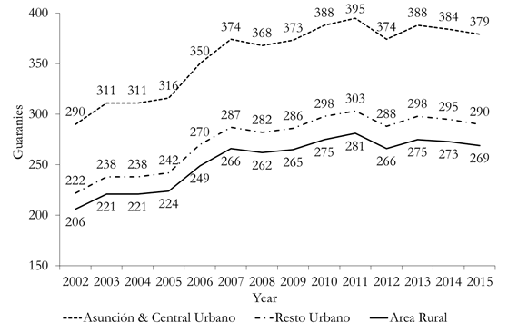
To complete this context of poverty reduction, it should be noted that extreme poverty lines (also called ‘food poverty lines') are updated annually using the food consumer price index for the Metropolitan Area of Asuncion. This index is provided by the Central Bank of Paraguay (BCP)⁹. Figure 4 presents the evolution of the real value of the extreme poverty lines adjusted by the general consumer price index. Food prices have grown at a faster rate than general prices, as reflected by the ascending value of the food lines. Food prices, relative to overall prices, were relatively stable until 2005 but soared in 2005-2007, in line with the evolution of world prices of many staple food commodities. Since 2007 the growth in food prices slowed down relative to other prices. By 2013, the extreme poverty line remained slightly higher than five years earlier.

Source: DGEEC and own calculations.

Notes: All values in this figure are expressed in thousands of Guaranies and in real values of October 2015.

Figure 4: Evolution of extreme poverty lines  

3. Data

In this paper, we use three sources of information. The 2011-2012 EIC-CV that contains detailed information on household expenditure on food and non-food items as well as detailed income data, including an agricultural module. This survey was carried out by the National Statistical Office from Paraguay (DGEEC for its acronym in Spanish) during a whole year from August 2011 to July 2012 and collected information for 5,417 households from both urban and rural areas. Its design allows doing robust estimations for urban and rural areas, and also for the departments of Asuncion, San Pedro, Caaguazu, Itapua, Alto Parana, Central and rest of departments (this includes all the remaining areas)¹⁰.

Secondly, we use comprehensive monthly price data at item level for the period 2007-2015. This data feeds the Consumer Price Index (CPI) published by the Central Bank of Paraguay¹¹. The general CPI includes 450 items, 359 goods, and 91 services. Of these, 127 are used in the food CPI. Item weights for both general CPI and food CPI allow us grouping individual items into sub-groups, such as Oils and Butters, Cereals and related products, Meat, Fresh and canned vegetables, among others¹².

Finally, we exploited the 2015 EPH. This survey is also carried out by DGEEC and generally used to estimate official poverty and inequality figures. It contains detailed information on income including labor, and various sources of non-labor income such as rents, interest or dividends, remittances (both internal and external), pensions, among others. In addition, unlike the EIG-CV, the EPH contains information related to existing social programs like Tekoporã (a conditional cash transfer program to families with school-aged children) and Adultos mayores (non- contributory pension plan which contemplates a monthly monetary transfer equivalent to one-quarter of the current minimum wage). We use this survey to simulate alternative policy responses that are presented and discussed in Section 7.

4. Do rural prices move similarly to those in Asuncion?

The Paraguayan CPI is disaggregated into several sub-components such as food, clothes, public services, health, and transport costs¹³. Prices are only collected in the metropolitan area of Asuncion. Thus, it is not possible to monitor price changes neither in the rural/urban spectrum nor at the departmental level, as it is possible in various other countries in the region (such as Brazil).

The CPI is used to annually update the value of national (extreme and moderate) poverty lines. For this purpose, both the food price index and the general price index are used. The assumption is that while price levels might differ across regions or areas of the country, price changes (inflation) are relatively similar across the country. This is a reasonable assumption in cases where transport costs are relatively low and distribution systems are highly developed, though less true in developing countries (^{Deaton, 1997}). Having access to unit values (even if imperfect substitutes for prices) for different areas and over a whole year, allows us to test (at least to some extent) whether the assumption is a reasonable one. Before moving into the analysis, a few caveats are in place. First, unit values are different from prices. Unit values are the implicit prices reported by households when asked about the quantity (i.e., in kilos, or grams) and total expenditure on goods. These values are affected by the quality (i.e., a kilo of prime rib costs more than a kilo of ground beef) and by the shop place (i.e., small shop or large supermarket), which could vary across the country. There are also measurement errors, especially when some information (on quantity or expenditure) is missing for a given good. Second, the survey was not ex-ante designed to provide accurate price estimates for sub-periods (months, trimesters, etc.) but for the whole year, therefore the representativeness by rural/urban areas for these sub-periods is not assured. Nonetheless, the distribution of interviews across months by urban/rural as well as by socioeconomic status is relatively smooth across time.

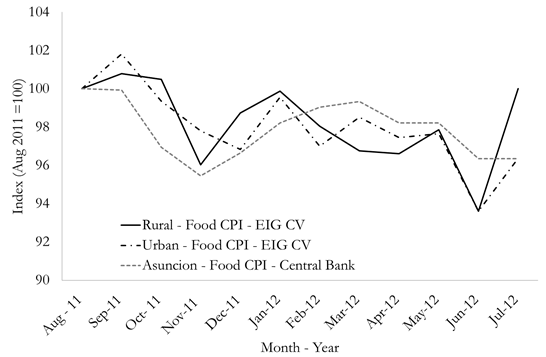
Based on the item weights used by the BCP for the CPI's construction and unit values from EIG-CV we generated monthly price indexes, for both urban and rural areas. A preliminary analysis suggests that (a) urban and rural price indexes move quite closely across the year; and (b) that both are close to the food price index reported by the Central Bank. The implication is that the assumption used to update the poverty lines is, at least for the period under analysis, not at odds with the information coming out from unit prices gathered at the household level. For our purpose, the remaining implication (c) is that it would not be inappropriate for the analysis that follows to use the CPI-BCP information to produce simulations using the EIG- CV (Figure 5).

Source: BCP and own calculations using EIG-CV 2011/12.

Notes: The Central Bank's Index refers to the official CPI used in Paraguay; while the other two alternatives are two indexes that try to mimic the official one based on the EIG-CV 2011/2012.

Figure 5: Evolution of urban, rural and CB indexes 

5. Analytical Framework

The idea that we explore in this paper is the following. Households consume a set of goods at a given set of prices. On the one hand, a price increase makes households poorer since with the same income they can buy fewer goods (expenditure effect)¹⁴. On the other hand, households could benefit from higher income if they work (e.g., farm-holders that produce and sell their own production or as wage employees) in those activities affected by the increase in prices (income effect).

The general analytical framework to explore the idea is the traditional agricultural model proposed by ^{Singh et al. (1986)}, continued among others by ^{Deaton (1989)}. In this paper, we closely follow the adaptation by ^{Brambilla and Porto (2009)}. The unit of analysis is the household, indexed by h. In equilibrium, household expenditures (including savings) e^h are financed with household incomes (including transfers).

In (1), goods (household members) are indexed by i (j). On the left-hand side, the expenditure function e(.) of household h is defined as the minimum expenditure that guarantees a given level of utility u^h. It depends on a vector of prices of consumption goods p, on the level of utility u^h, and other household characteristics x^h (i.e, household composition). Income comprises the sum of the wages of all working members j (w_j) and the sum of the profits (π_i) made in different economic activities i. Profits include the net income from agricultural production or farm enterprises as a function of prices, technology, and some key household characteristics (summarized by φ). T^h measures transfers (public or private), savings, and another unmeasured factor returns. Finally, x^h represents an exogenous income. It is evident that household welfare depends on equilibrium variables such as prices and wages (that affect household choices) and also on household endowments¹⁵. It follows that changes in commodity prices affect welfare directly via consumption and production decisions and that these impacts depend on household choices and endowments.

Let's consider now the impact of changes in the price of commodity i, which can be obtained by differentiating equation (1) -while keeping utility constant and adjusting T^h. It follows that

where CV ≈ −dx0e is a measure of the compensating variation, as a share of initial expenditures¹⁶. In equation (2), b_i is the share of total household income from the production of good i, and s_i is the budget share spent in good i. εwij  is the elasticity of the wage earned by household member j with respect to the price p_i ·- θ_j is the share of the wage income of member j in total household income¹⁷. The right-hand side of (2) reveals impacts on both household expenditure and income. In a first-order approximation, the first term reflects that there is a direct impact on profits if households produce the good i, which depends on the share of total household income attributed to this good, b_i. The first term also measures, through budget shares s_i, how prices affect the consumption side. It is clear that households that are net-consumers (b_i < s_i) are worse off if prices go up whereas net-producers (b_i > s_i) are better off. The opposite is true for price reductions. The second term represents a first-order approximation of how price changes affect wages. Against a price change, labor demand for different types of labor (an also labor supply) can change, thus affecting equilibrium wages. This response is captured by the elasticity εwij . These impacts on labor income depend also on the share of total household income contributed by wages of different household members θ^j18.

As argued by ^{Brambilla and Porto (2009)} and ^{Lederman and Porto (2016)}, many issues associated with the first order impacts need to be highlighted. First, the role of imperfect pass-through of international to domestic prices and therefore to households¹⁹. Second, the existence of spillover effects both on the production and on the expenditure side²⁰. Third, while the net-consumer/net-producer approach is very intuitive, it rests in a strong assumption: the first-order approximation. Relaxing this assumption or analyzing large price changes, require the consideration of responses in demand and supply (second-order effects)²¹. As we previously mentioned, consumers always lose from a price increase. But if they can adjust, the losses can be ameliorated by reducing purchases of the more expensive goods²². The addition of second-order effects alters equation (2) as follows:

where the last term S(Δp) corrects for substitution behavior, as a function of the full vector of price changes²³. The literature has tried to quantify consumption responses through the estimation of a system of demand elasticities (own- and cross-price elasticities)²⁴. ^{Friedman and Levinsohn (2002)} -while did not include wages or income responses in their model- found that allowing for substitution effects in consumption makes a big difference and the estimated losses can be cut by a half. Nonetheless, the distributional consequences are shown to be rather stable across the whole income distribution. In a recent study, ^{Tiberti and Tiberti (2018)} indicate that the second-order effects reduce the negative effects due to the first-order consumption effects, with significant differences across quintiles. On average, the second- order effects represent up to roughly 40 percent of total first-order effects.

As discussed by ^{Ferreira et al. (2013)}, and to the best of our knowledge, there is still no evidence that has fully captured all terms of equation (3). This paper is not the exception. Unfortunately, due to the lack of data to estimate substitution in consumption against a price change we are not able to include second-order effects. In any case, not including substitution effects lead us to estimate an upper bound for the effect on poverty and inequality of price changes.

6. Simulation and Main Results

6.1. Simulation

Between September 2010 and August 2011, prices of food items in Paraguay rose 17 percent, whereas overall inflation was around 9 percent (5.4 percent if we do not include food items)²⁵.

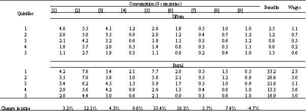
About 40 percent of the total population lives in rural areas, where a sizeable part of incomes is related to agriculture. Therefore, the potential impact of food price changes on poverty and inequality might be significant. To shed light on this, we simulate an increase in prices similar to the previously mentioned one (Figure 6). In the simulation, we consider to some extent the heterogeneity of price changes observed across foodstuffs. The EIG-CV data allow us to observe 127 food items prices, which we grouped into nine food groups, following the classification used in the construction of the Consumer Price Index²⁶.

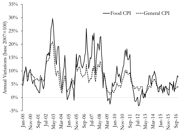
Source: Central Bank of Paraguay.

Notes: The food share presented in this figure corresponds to the moving average of each centile. Urban and rural centiles are constructed using the population living in each area respectively. Naturally, national centiles consider the population of the whole country.

Figure 6: Annual variations in the food and general price index 

We calculate the first-order effect of this price change as described by equation (2). Regarding the first term of equation (2), available information on household expenditures and incomes (provided by the EIG-CV) allows us to compute both consumption and production shares. Specifically, in our view, the calculation of production shares represents an important contribution of this paper, considering that some relevant studies do not calculate it due to a lack of information²⁷. Moreover, Paraguay has the greatest share of rural the population in Latin America and, as a consequence, own production is a key determinant of household’s welfare. As we will appreciate later, omitting this component of the income effect does not have negligible effects on the final results. Regarding the wage-price elasticity (εwij ) for the second term of the right-hand side of equation (2) we initially assume a value of 0.2, based on ^{Ravallion (1990) 28}. Given that this election is, to some extent, arbitrary we explore other alternatives for sensitivity analysis (as, for example, in ^{Ferreira et.al. (2013)}). Specifically, we consider the following cases: i) no response (εwij  = 0), ii) long-run response (εwij  = 0.5) and iii) full transmission (εwij  = 1.0)²⁹. Finally, we assume that (consumed and produced) quantities of each item are the same before and after the price change. Then, we compute the resulting household level values of expenditure and incomes and analyze the welfare variation across the income distribution. As mentioned, this implies an upper bound effect, given that households may substitute either in consumption or in production.

6.2. Main Results

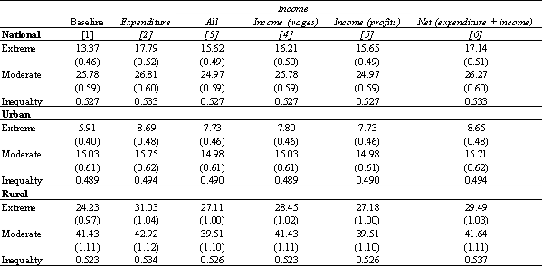
We begin by presenting the results on the expenditure effect. Considering that prices of food items increased relatively more than the general level, this effect is majorly explained by the share of expenditure that households spend on food. Naturally, as expected, this share varies across centiles of income per capita, and between urban and rural areas with an average of 37 percent and 47 percent, respectively (Figure 7). This is a standard textbook result and is well known as the Engel curve. Our result suggests that the expenditure effect is negative and obviously regressive everywhere, but larger in rural than urban areas (Figure 8). When comparing extreme poverty rates after the simulated price hike, and considering only the expenditure effect, we can appreciate an increase in the number of people not able to afford the basic food basket³⁰. This increase in extreme poverty is greater in rural areas (Table 2). Specifically, extreme poverty increases three points in urban areas and more than six points in rural ones. Something similar occurs with moderate poverty that rises approximately half a point in urban areas but more than a point and half in rural areas. Inequality rises slightly.

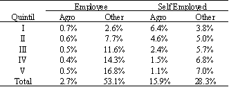
On the other hand, the food price hike leads to higher incomes for small farm holders and those employed in agriculture. The income effect that we address in this paper includes not only the effect of prices on wages, as in ^{Ferreira et. al. (2013)}, but also greater returns for agriculture entrepreneurs and self-employed. We identified agro- and non-agro-related household income, and estimated the income effect only on those working in agro-related activities³¹. As with the expenditure effect, differences across areas are substantial; the probability of having an agricultural-related income is 17 percent in urban areas whereas 65 percent in rural ones³². Table 2 presents the overall income effect, differentiating between income-wage effect and income-profit effect. Both effects lead to a reduction in poverty but while the income-wage effect is quite small, the income-profit effect significantly contributes to poverty reduction. In addition, the income-profit effect is greater in rural areas. Two results are important to be highlighted. First, the fact that the income-wage effect is negligible reveals that the agro-industrial sector is still something not very well developed in Paraguay Therefore, improvements in this sector will then help to boost household income and contribute to poverty reduction. Second, not including the income-profits effect, as in ^{Ferreira et al. (2013)}, leads to an important omission in total household income. This component may also be more important in Paraguay as compared to other countries in Latin America, given its employment distribution³³.

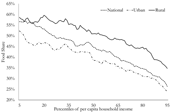
Source: Own calculations based on EIG CV 2011/12.

Notes: The food share presented in this figure corresponds to the moving average of each centile. Urban and rural centiles are constructed using the population living in each area respectively. Naturally, national centiles consider the population of the whole country.

Figure 7: Food share on total expenditure by area 

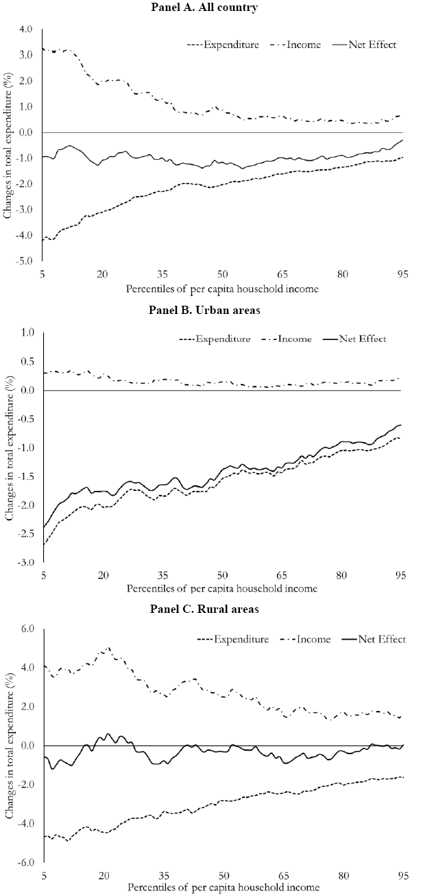
Source: Own calculations based on EIG CV 2011/12.

Notes: Each effect in these figures was estimated as the moving average of each centile.

Figure 8: Expenditure, Income and net effect (price elasticity = 0.2) 

Table 2 Extreme and moderate poverty, and inequality (price elasticity = 0.2) 

Source: Own estimations based on EIG CV 2011/12.

Notes: Standard errors in parentheses. Extreme and moderate refer to the headcount ratio using the extreme and moderate poverty line respectively. Inequality refers to the Gini coefficient. In this table we consider a price elasticity of 0.2 and full pass-through of profits linked to self-employed earnings. In each column we report the following concepts: [1] baseline estimation (before the shock); [2] estimates after shock where we include only the expenditure effect; [3] add to [1] the income effect; [4] add to [1] the wage effect; [5] add to [1] the profits effect; [6] add to [1] the expenditure and income effect.

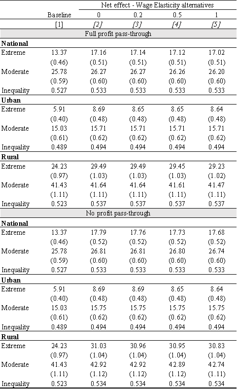
As Figure 8 suggests, the income effect is positive and progressive in rural areas and negligible in urban areas. As we increase the wage-price elasticity (εwij ), the income effect becomes greater. But wages do not play a substantial role as can be observed in Table 3, which presents a summary of additional estimations with alternative values for εwij . Overall, at the national level, we find that the potential impact on the welfare of an unexpected increase in food prices in Paraguay is a very flat U-shaped curve (Figure 8) ^34,35. Using the same logic as ^{Higgins and Lustig (2013)}, Table 4 presents a mobility matrix at the national level and by area. It shows in a dis-aggregated way, the initial composition of socioeconomic classes before and after the price shock (including both the expenditure and income effect). For instance, 30 percent of individuals that were under moderate poverty before the shock, fell into extreme poverty after the price variation.

Table 3 Summary of simulations: elasticity and pass-through of profits alternatives 

Source: Own calculations based on EIG CV 2011/12.

Notes: Standard errors in parentheses. Inequality refers to the Gini coefficient. In each column we report the following concepts: [1] baseline estimation (before the shock); [2] estimates after shock where we consider a wage elasticity of 0 in [2], 0.2 in [3], 0.5 in [4] and 1 in [5], respectively.

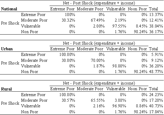
Table 4 Mobility Matrix before and after the shock (simulation) 

Source: Own calculations based on EIG CV 2011/12.

Notes: This table should be read from left to right. For instance, for those individuals that were in an extreme poverty status in the pre-shock situation, after the shock (simulation) some of them ended up in the same situation (extreme poverty), while others move to moderate, vulnerable, or non-poor status. Values in this table are based on a simulation that considers a price elasticity of and full pass-through of profits linked to self-employed earnings.

7. Policy Responses: simulating in-cash-transfers interventions

As was shown in the previous section, a shock on food prices increases poverty rates. To mitigate this perverse effect, governments can use their social protection systems³⁶. Tekoporã is the most important social program in Paraguay, devoted to improving life’s quality of the most deprived. This program warrants food access, health, and education to less well-off families. Also, it strengthens social networks to eradicate the inter-generational transmission of poverty Its design is pretty similar to many other conditional cash transfer programs that were implemented in the region. It is mainly focused on families in extreme poverty and vulnerability, which have children and adolescents between 0-18 years old, disabled persons, and pregnant women³⁷.

Tekoporã has been gaining relevance and coverage since 2005 and its beneficiaries have increased steadily. In 2005, 4,324 families in poverty and vulnerability conditions were covered by the program. Actually, the program covers all departments in Paraguay with 131,159 families³⁸. Each household receives a lump sum transfer of Gs. 90,000 and a flexible transfer depending on the number of children (of Gs. 40,000 for each child). For instance, a household with four children receives a total amount of Gs. 250,000³⁹.

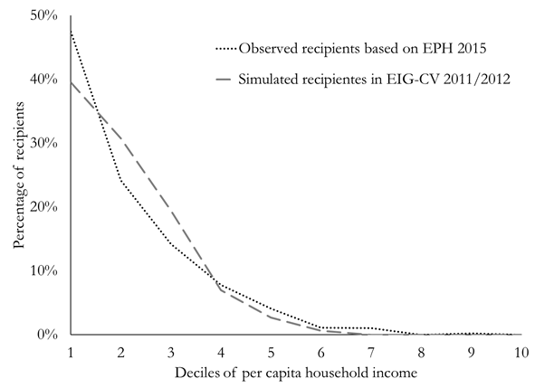
The existence of Tekoporã, allows us to simulate a policy response from the government side to help those most affected by the price shock⁴⁰. To assess this issue, a major methodological obstacle needs to be removed. In particular, the main source of information used in this paper (EIG-CV 2011-2012) does not report a specific question about whether the individuals receive or not the program. So, an approximation to a hypothetical distribution of Tekoporãs beneficiaries needs to be estimated. For this purpose, we take advantage of the EPH 2015 where a specific question about the reception (or not) of Tekoporã is reported. We followed several steps outlined below.

First, we identify the current number of households receiving Tekoporã in EPH 2015. Second, we propose a probabilistic model to identify those simulated beneficiaries in EIG- CV 2011-2012 but based on EPH 2015. Specifically, we run a probability model (see Table A3 in the Annex) using as a dependent variable whether the household receives the program or not. As regressors, we include a set of household head characteristics and a set of variables that captures the household structure and dwelling features⁴¹. Thus, through this model we obtain the estimated probability of being Tekoporã beneficiary in EPH 2015⁴². Third, using the previous model coefficients we compute the estimated probability in the EIG-CV 2011-2012, and we obtain a simulated distribution of hypothetical beneficiaries^43,44. We set the number of beneficiaries in the EIG-CV 2011-12 to be the same amount as those in EPH 2015.

Afterward, using the current Tekoporã's scheme and the mimic of beneficiaries in the EIG-CV 2011-2012, we simulate governmental assistance through an additional transfer to Tekoporã's beneficiaries. This additional amount is calculated as a share of the actual (monthly) transfer that beneficiary's receipt. Regarding this, we proposed two scenarios (not exhaustive, logically). One in which each household receives an extra monthly transfer. Another in which each household receives four extra transfers. So, following the previous example, a household with four children receives (in our simulation) a monthly compensation of Gs. 250,000 and Gs. 1,000,000 in each scenario⁴⁵.

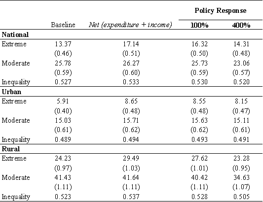
The last two columns in Table 5 present the simulations (we keep the first two columns as in Table 2 for reference). The first of them generates a small decline in (extreme and moderate) poverty rates. Also, inequality is reduced after the price shock (column 3 versus 2). This reduction is almost imperceptible in urban areas while much greater in rural areas (moderate poverty is even lower than before the shock)⁴⁶. The second scenario generates more pronounced declines, logically, as the transfer is four times bigger. At the national level, extreme poverty is reduced by three points reaching almost pre-shock values. Even moderate poverty is two points less than before the shock. Again, much of the action is coming from rural areas while almost nothing happens in urban ones. In urban areas the transfer does not compensate enough those households that were affected by the price shock, ending with extreme poverty higher than the baseline scenario^47,48.

Table 5 Policy response simulations 

Source: Own calculations based on EIG CV 2011/12.

Notes: Standard errors in parentheses. Inequality refers to the Gini coefficient. In this table we consider a price elasticity of 0.2 and full pass-through of profits linked to self-employed jobs. The policy response refers to either one or four extra monthly payments of Tekoporã.

8. Conclusions

In this paper we contribute by providing evidence of the potential effects on welfare of a price increase, disentangling between those that affect consumption and those that affect production. The paper also differentiates the effects between rural and urban areas. We focus on Paraguay where the agricultural sector plays a key role and where the availability of data is far from being the ideal one, which imposes challenges to the analysis.

Concretely, we simulate a food price hike of approximately 17 percent, similar to the one experienced in Paraguay between September 2010 and August 2011. Using micro-level data, we estimate the impact of this hike on households' welfare. We use the Income and Expenditure (EIG-CV 2011-2012) and the Permanent Household (EPH 2015) surveys. In addition, we use detailed monthly price data collected in Greater Asuncion gathered by the Central Bank of Paraguay The analytical framework is based on the compensating variation, assuming that households are entitled to their pre-shock level of utility. We consider three different effects: the expenditure effect, as consumers face more expensive prices; the income effects, derived either as greater wages for employees in agricultural activities or as greater profits for those self-employed; and the government policy response, simulated as an increase in the cash transfer to beneficiaries of the existing social program Tekoporã. Here, we contribute by estimating a sub-component of the income effect (i.e., the profit effect) that was not considered in the existing literature (at least for Latin American countries). This contribution is relevant since the profit effect explains a substantial part of the final results, given the economic structure of Paraguay. One caveat of our results is that we were not able to estimate behavioral responses after the shock (i.e., second-order effects). Given this, we think that our results could be understood as upper bound estimates, where households have no room to adjust consumption or production decisions.

Our results show that the effects of higher food prices on poverty and inequality could be non-trivial, particularly for those in rural areas. Specifically, we find that the potential overall impact of an unexpected increase in food prices in Paraguay could be represented by a very flat U-shaped curve effect. This means that if we were to sort the population from the poorest to the richest, those households located in the extremes of the distribution will be less affected (though the differences throughout the distribution are not large). Yet, governments such as Paraguay, that have in place a relatively extensive social assistance system could take measures to react quickly to such shocks, protecting the most vulnerable. The paper simulates such policy response, with varying generosity degrees on the transfer.