


 Inglés (pdf)
 Articulo en XML
 Referencias del artículo
 Enviar articulo por email
 Citado por SciELO
  Similares en
SciELO
Similares en
SciELO 
 Permalink
1. Introduction
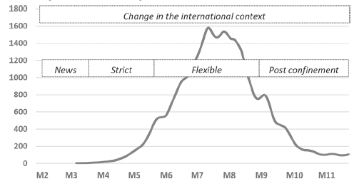
News about the pandemic originated by the coronavirus (SARS-CoV-2) reached Bolivia in February 2020. The first two confirmed cases were registered on March 10 and the first three deaths were registered on March 28. By March 17, the government declared a national strict quarantine, extended twice and ending May 10. The so called “dynamic and conditioned” or simply flexible quarantine began May 11, extended twice and ended August 31. Post confinement recommendations began immediately after in September. Figure 1 shows the entire period of the shock to the Bolivian society and economy, beginning the moment of the COVID-19’s news arrival in February and into the average daily change of COVID-19 cases in its first wave, with peaks in July and August, to its ending by November 30 with an accumulated 144,708 cases (8,957 deaths, 121,702 recovered and 14,049 active). The pandemic’s second wave began immediately after in December and continued over into 2021. This article concentrates only on the first wave’s 10-month shock to the economy from February to November 2020.
Government decisions at the national and subnational levels, as well as decisions by civil society down to every family and person, all subject to their own restrictions, initially sought self-protection to avoid contagion and loss of life, particularly from March to May. However, the very same decisions had a predictable but inevitable secondary effect, that of loss of economic activity, which in most cases meant loss of household income particularly of the self-employed and in many cases it meant unemployment. The government tried to alleviate the loss of income from the strict quarantine with several cash transfers, however it soon became evident not only that the amounts transferred would not be enough but the transfers themselves would not be a financially sustainable strategy. Complementary policies were also issued directed at alleviating the costs of producing and living which helped in sharing of the welfare loss with other economic actors (banks and rentiers) at least for some time. Later decisions by government, organized civil society and individuals, particularly from June to the end of the year, were to rather let each search for their own best equilibrium between health and work. Decisions that changed rapidly based on the observed behavior of the pandemic itself. Simultaneously there was a myriad of other actions by subnational governments and organized civil society, as well as many stories of adaptation, entrepreneurship and collaboration. This brief description of how Bolivian society reacted to the pandemic is an important part of the same shock to the economy contained within Figure 1 during the 10 months of the first wave from February to November. It reflects a society facing the unknown particularly in the early months of the first wave, expressing its fears but also taking risks in testing its limits, and later in the year learning from own accumulated experiences and from the experiences of others.
Internationally the COVID-19 pandemic affected all countries, directly and indirectly, as each reacted in different ways to find their own best equilibrium between protecting their citizens’ health from cross border contagion and at the same time maintaining supply chains and different degrees of trade activity which adapted to changing policy conditions connected to the evolution of COVID-19 in each country and throughout the world, therefore affecting global travel, transportation, prices and trade. This is also part of the shock experienced by the Bolivian economy, like all other countries, expressed in drops in the value of exports and imports as well as changes in capital flows. The world was caught by surprise but early in the year there were international announcements for the beginning of vaccine research and development whose potential efficacy was unknown only until the end of the year1.
Summarizing, the COVID-19 pandemic shock is understood here as comprising COVID’s contagion dynamics, fear of contagion dynamics and policy as well as their interactions. The latter expressed in world reactions as well as within country reactions by government, civil society, families and individuals, which in turn have impacted the functioning of the economy in every country along with impacts on all society’s affairs beyond economics. This paper begins with the belief that the net economic effect from the COVID-19 pandemic shock to the Bolivian economy has been ultimately captured in the Bolivian Monthly General Economic Activity Index (IGAE in Spanish), published by the Bolivian National Institute of Statistics (INE in Spanish). Based on this index, the purpose of this paper is first to graph and measure the magnitude of COVID-19’s impact on the overall Bolivian economic activity and second, graph and measure the magnitude of COVID-19’s impact on every economic sector.
The methodology conceives COVID-19 as a natural experiment and analyzes it from a time series perspective by seeking to measure the distance between the time series of the observed economic activity with COVID, to the time series of its counterfactual without COVID. The counterfactual is built from a forecast of economic activity without COVID using ARMA-type time series models based on all past information, previous to the pandemic, therefore producing a counterfactual average series within confidence intervals. The objective is modest in the sense that the resulting impact measure includes all changes in the macro and micro economy caused by COVID-19 as well as all policy and society’s reactions to the disease, without identifying which actions worked better than others or discussing pre-COVID conditions or governance quality by economic sectors, but rather to simply record the graphical behavior of both the observed and the counterfactual series for its visualization and compute their accumulated distance as a measure of the impact’s magnitude.
Key results are that the difference between the observed and average counterfactual time series show a 12.64% loss in overall economic activity during the first wave’s 10-month period from February to November, with a tilted W-shape short-run recovery. The breakdown by the economy’s twelve sectors shows the communications and agricultural sectors did not experience any impact but rather were highly resilient. While the rest on average simply lost, with minerals -34.94% and construction -34.49% the most damaged, followed by transportation -20.91% and restaurants & hotels -20.68%, manufactures -14.79% and commerce -12.04%, finance -9.53% and utilities -9.12%. The impact on the oil & gas and government sectors could not be determined. A high recovery rate across sectors did happen however characterized by heterogeneity in the sense that most did not follow the overall economy recovery shape, but rather followed different speeds, times and magnitudes thus affecting economic connections across sectors to some unknown degree.
Besides the monthly IGAE data, INE also publishes the monthly rates of variation and the monthly accumulated rates of variation for the overall economy and all economic sectors. However, the accumulated measures produced in this paper differ in three fundamental ways from those produced by INE. First, the reference for computing variations is the counterfactual rather than the observed data 12 months ago, noticing that both respect the natural seasonality in the data resulting from the Bolivian economic structure. Second, the counterfactual for 2020 is produced from a forecast based on all past information, therefore it also captures the decreasing growth tendency that would have been observed in 2020 assuming no fundamental change in the economic context and policies. Up to 2019 this context was characterized by a twin fiscal and balance of payments deficit resulting from the end of the economic boom since 2013, parallel to the end of high international commodity prices. Similar assumption is implicitly made by INE but applied to the observed data 12 months ago as its reference, therefore not including the growth tendency that would have been observed in 2020. Third, INE’s accumulated rates of variation are not provided within confidence intervals. As a result, the average numbers produced in this paper tend to be higher compared to those produced by INE with key additional gains, that of a better graphical visualization of the impact’s cumulative magnitude and monthly evolution in relation to the overall economy, by economic sectors and within confidence intervals.
A related concept in the macroeconomic literature is that of potential or full employment output meaning the maximum amount an economy can produce in the long run (Williams, 2017). Its forecast has important implications for macroeconomic policy analysis depending on the sign and magnitude of the output gap or the difference between the forecasted real and potential outputs. However, the counterfactual concept and impact measure used in this paper differs in three fundamental ways. First, forecasting potential output is an effort at predicting the future tendency and magnitude of the output gap while the counterfactual is an effort at measuring the impact of a past event. Second, potential output prediction tends to be a smoothed version and forecast when based either on the observed medium and long term behavior of the series or on a theoretical construct heavy on assumptions, while the counterfactual in this paper, on the contrary, seeks to forecast the short-term during the period of a particular past event based on the short, medium and long-term behavior of the series before the event. Third, potential output must be updated frequently as new information arrives in order to improve accuracy of predictions while the counterfactual does not need to.
Besides this introduction, section 2 explains the data and methodology in more detail, while sections 3 and 4 present the pandemic’s impact measure and graphical visualization by economic sectors and overall economy. The last section summarizes along with final comments.
2. Methodology and data
A natural experiment is an event or intervention whose circumstances were not under the control or manipulation of researchers, but where interpretation of evidence and causal inference must be drawn with care due to potential lack of randomness (Craig et al., 2012). This perspective of a natural experiment requires pre shock and post shock observations, where a clear identification of comparable treatment and control groups is necessary. The COVID-19 pandemic is unique and can be understood as a natural experiment, however, given that its effects on the world economy have been so large, wide and profound at the same time, it has simply affected everyone and everything directly or indirectly by generating a cascade of multiple interacting changes in world society, well beyond the purely economic sphere but including it. For this reason, a pure control group does not really exist under the traditional randomized control trial perspective particularly if the objective is to measure the overall economic impact of COVID-19 for a country.
As an alternative this paper’s proposal is to adopt a time series perspective. When the time series of an aggregate economic variable like IGAE experiences a shock it automatically generates two paths, the one affected by the shock and expressed in the actual or observed behavior of the series and the one that the time series most probably would have followed if the shock did not happen or counterfactual. The counterfactual is strictly obtained from the best forecast of the series based on all its past information and behavior resulting in the most likely path among the many possible. The cumulative distance overtime between these two series would be the natural measure of the shock’s impact. This way of computing impact has the advantage of not requiring that the shock itself be expressed in a complex set of treatmenttype variables that must enter a regression equation.
Three important caveats are needed to complement the argument. First, for true impact attribution it must be observed that no other unrelated shocks impacted the same time series at the same time (like the November 2019 political shock that could have been carried over to 2020) or at least it should be possible for those other shocks to be controlled away. Second, the effects of all planned or unplanned changes in society’s behavior directly or indirectly related to the original shock (COVID-19 pandemic) are captured within the outcome variable IGAE and therefore are already considered part of the impact measure without need to separate the contribution of each and every change. Third, time series must be long enough and their characteristics of non-stationarity and autocorrelation in the mean and variance must be considered and treated with care for reliable average measurements and their confidence intervals.
This perspective falls within the quasi-experimental class of interrupted time series (ITS) analysis mostly used in health policy research (Hudson et al., 2019), but where the problems of non-stationarity, autocorrelation and seasonality must be taken into account (Schaffer et al., 2021). However, instead of computing impact as changes in the level and trend of the outcome variable, the proposal here is to compute the accumulated distance between the observed and counterfactual series.
This paper uses ARMA-type models to forecast a key economic time series based on all of its past information, previous to the external shock, in order to obtain the counterfactual path or time series under the assumption of no shock. ARMA models were popularized by Box and Jenkins (1970)) and Box, Jenkins and Reinsel (1994) for time series analysis and forecasting. A key advantage of ARMA-type models is their ability to capture the natural regularities in a time series by way of the autocorrelation and moving average contained in it as well as seasonal operators. Other advantage is the possibility to include deterministic-type variables like seasonal dummies that can also help capture natural regularities contained in the data or in some cases explain extreme observations, and tendency-type variables that can help capture natural linear or quadratic trends in the data. An additional advantage of these type odels is their natural expansion to GARCH-type models in case observed volatility in the time series is an issue. ARCH and GARCH models where originally introduced by Engle (1982) and Bollerslev (1986) respectively, and have evolved into many different variants over time.
The following is a presentation of the basic ARMA (p, q) - GARCH (r, s) model:
The first expression is an ARMA model or equation of a stationary time series
The econometric strategy in the context of the IGAE times series of the overall economy index and the sector indexes that compose it, in a first stage, is to estimate ARMAGARCH models for the stationary transformation of each of them individually in search for parsimonious models with highest R-square and normally distributed white noise residuals in their mean and variance, and in a second stage use each model to forecast the levels of each time series index for the period of interest. This forecast would be referred to as the counterfactual or without COVID. It is expected that each sector and overall indexes will produce specific models adjusted to capture own seasonal and structural particularities, however it is expected that most models will not require estimation of a GARCH process. The minimum mean squared error forecast is the conditional expectation and forecasts into the future are computed recursively based on the model equation. A prediction interval is also desirable for each point forecast to establish significance.
In a third stage, the strategy is to produce a graphical representation of the counterfactual against the observed times series index with COVID to visualize the magnitude of COVID-19’s impact as well as against the graph of variations of COVID cases (with planned and unplanned society’s reaction within it) for graphical visualization of the moments of greater impact. The measure of COVID-19’s impact itself is computed as a percent loss of economic activity which would be the difference between the observed and counterfactual time series in levels applied to each sector and overall indexes during the period of the first wave from February to November 2020.
Regarding data sources, the IGAE time series (overall and by sectors) can be freely downloaded from INE’s webpage (link provided in the references), which also contains its methodology and sources of information. The series was preliminary when first published up to November 2020. The COVID-19 data can be freely downloaded from Bolivia Segura’s webpage (link provided in the references).
3. COVID’s impact on overall economic activity
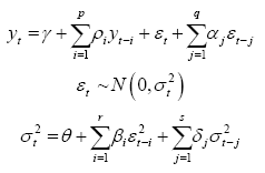
The monthly rhythm and evolution of the Bolivian General Economic Activity Index (IGAE) is presented in Figure 2 showing some characteristics: First, it has been growing at an annual average rate of 3.95% for the five-year period from 2015-2019, although with a decreasing tendency since 2013 as shown by the monthly growth rate of a Hodrick-Prescott smoothed IGAE series (HP rate) up to December 2019 (right axis). Second, the index follows an annual regularity or seasonality with January, February and March, the months of low activity, from April to August, the months of intermediate activity, and from September to December, the months of high activity. Third, there is a noticeable significant break in its tendency and seasonal pattern starting February 2020 caused by COVID-19.
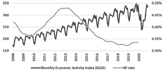
The question is how the IGAE series would have looked like or would have behaved if COVID-19 pandemic didn’t happen. This is the counterfactual series needed only for the period from February to November 2020. Following the econometric strategy presented above, the order of integration and estimated model for the global IGAE index are presented in Annexes 1 and 2. Figure 3 is the result of the exercise where the dashed line shows the first wave of monthly variations of confirmed COVID-19 cases, reaching its maximum between the months of July and August, while the previous months from mid-March to early May were of strict quarantine. The IGAE with COVID line corresponds to the evolution of IGAE as it was observed and registered by INE, including the November 2019 political conflict and the pandemic experience from February to the end of November 2020, when the first wave ended (the second wave began immediately after in December 2020). While the IGAE without COVID line is a forecast from November 2019 to November 2020 representing how the IGAE index would have behaved if neither the political conflict nor the pandemic had occurred. The forecast begins in November 2019 rather than February 2020 in order to eliminate the potential contamination from the November political conflict that impacted the economy that month and whose economic consequences might have been carried over onto 2020.
Figure 3: COVID’s impact on overall IGAE Variations in COVID-19 cases are measured on the right axis.Source: Author’s elaboration based on data from INE and Bolivia Segura.
The visual difference between the IGAE with and without COVID lines shows the magnitude of the pandemic’s impact on the Bolivian economic activity for the period of ten months between February and November 2020. The series with COVID changed starting February, showing a significant fall of economic activity particularly between April and May, during the strict quarantine; a fall in a magnitude not experienced before in the history of the series. While the series without COVID within dotted confidence intervals is the counterfactual series that reproduces with precision the seasonal behavior and tendency that would have occurred without COVID-19, taking into account all past information of IGAE. The short-run recovery behavior began U-shaped, but because of the setback between June to August, when COVID-19’s contagion expanded and reached its highest peaks of registered cases, it ended with a W-shape tilted and prolonged to the right. The figure also shows the economic impact of the political conflict in November 2019 with an immediate V-shape recovery. The fact that the observed and counterfactual are basically the same in December 2019 and January 2020 provides some confidence that the rest of the observed series is free from that contamination during 2020, at least in the economic sphere but certainly was not so in the political sphere.
Computation of the impact itself is obtained by subtracting the line with COVID from the line without COVID; the area between what actually happened compared to what would have happened without COVID-19. This way of measuring impact is conceptually different to subtracting today’s observed value respect to its value 12 months ago. This last would not be a measure of impact since it does not take into account that the economy would have continued growing during 2020 at the rhythm and tendency it was growing given the domestic and international context and the economy’s structure. Table 1 shows the accumulated IGAE would have grown up to 3,315.64 points but grew only up to 2,896.66 which establishes the pandemic’s impact at an average accumulated -12.64% loss of economic activity in the period between February to November 2020.
Table 1 Computing COVID-19’s impact on overall IGAE
| Month | IGAE with COVID | IGAE without COVID | Points difference | Accumulated rate |
|---|---|---|---|---|
| 20M2 | 278.23 | 283.30 (±2*4.03) | -5.07 | -1.79% |
| 20M3 | 302.75 | 319.37 (±2*4.82) | -16.62 | -3.60% |
| 20M4 | 238.71 | 336.12 (±2*5.40) | -97.41 | -12.69% |
| 20M5 | 242.28 | 330.57 (±2*5.65) | -88.29 | -16.34% |
| 20M6 | 280.16 | 337.23 (±2*5.99) | -57.07 | -16.46% |
| 20M7 | 276.10 | 323.02 (±2*6.09) | -46.92 | -16.14% |
| 20M8 | 280.43 | 329.19 (±2*6.48) | -48.76 | -15.94% |
| 20M9 | 319.77 | 352.80 (±2*7.17) | -33.03 | -15.05% |
| 20M10 | 344.61 | 358.90 (±2*7.56) | -14.29 | -13.72% |
| 20M11 | 333.62 | 345.14 (±2*8.45) | -11.52 | -12.64% |
| Accumulated | 2.896.66 | 3,315.64 (±2*61.63) | -418.98 | |
|
Pandemic's impact => (95% confidence interzai) => |
-12.64% (-15.77%,-9.26%) |
|||
In parenthesis ±2*S.E. is a 95% confidence interval.
Source: Author’s elaboration based on data from INE.
4. COVID-19’s impact by major economic sectors
The IGAE index is also a weighted average of 12 major sectors of economic activity, each with its own index, therefore it is possible that all sectors might have experienced different degrees of economic activity loss due to the pandemic, different compared to the global, and it is also possible that some sectors might have benefited, or at least were more resilient than others. Following the same methodological approach of comparing observed behavior to its counterfactual from February to November 2020, this section presents COVID-19’s impact sector by sector. In every case, forecasts begin in November 2019 rather than February 2020 in order to eliminate the potential contamination of the counterfactual from the November 2019 political conflict that impacted the economy that month which might have been carried over to 2020 and impacted each sector differently. Following the econometric strategy presented above, the order of integration and estimated model for each sector are presented in Annexes 1, 2 and 3.
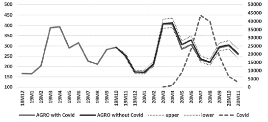
4.1. Agriculture
The monthly rhythm and evolution of economic activity in the Bolivian agricultural sector is followed by the Agriculture, Livestock, Forestry, Hunting and Fishing index (AGRO for short) within the IGAE index. This sector has been growing at an annual average rate of 5.61% for the 5-year period from 2015-2019, following an annual seasonality with March and April the months of highest economic activity and December and January, the months of lowest economic activity. How would the AGRO series have behaved if COVID-19 pandemic didn’t happen? Figure 4 is the result of the exercise where the AGRO with COVID line corresponds to the evolution of the agricultural sector as it was observed and registered by INE and the AGRO without COVID line represents how the sector index would have behaved if neither the political conflict nor the pandemic had occurred or counterfactual, within dotted confidence intervals. The visual difference between the two lines shows the small to negligible magnitude of the pandemic’s impact on the agricultural sector for the period of ten months from February to November 2020, with a clear difference concentrated only in May and June but fully recovering by July, while the months of March and April of highest sector activity were basically not affected by the strict quarantine months. The November 2019 political event didn’t affect this sector either. Computation of the accumulated difference establishes the pandemic’s impact at an average of -2.46% loss of economic activity for the period between February to November 2020. However, the range of the confidence interval (-8.16%, +4.00%) suggests the pandemic didn’t have an impact on this sector, thus the agricultural sector was highly resilient during the pandemic’s first wave.
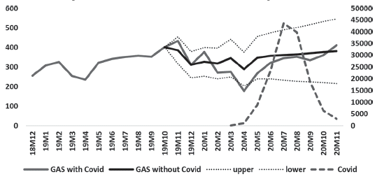
4.2. Oil and gas
The monthly rhythm and evolution of economic activity in the Bolivian oil and gas sector is followed by the Crude Oil and Natural Gas index (GAS for short) within the IGAE index. Growth of this sector has been decreasing at an average annual rate of -5.25% for the five-year period from 2015-2019, following an annual seasonality, at least up to 2017, with November the month of highest economic activity and February and April the months of lowest economic activity. The seasonal pattern was already broken since 2018 and became more volatile during 2019. How would the GAS series have behaved if COVID-19 pandemic didn’t happen? The observed volatility of the series since 2018 has made it hard to obtain a reliable model in this case, affecting forecast accuracy. Figure 5 is the result of the exercise where the GAS with COVID line corresponds to the evolution of the oil & gas sector as it was observed and registered by INE and the GAS without COVID line represents how the sector index would have behaved if neither the political conflict nor the pandemic had occurred or counterfactual. However, the width of the dotted confidence intervals produced for the counterfactual series is too wide and contains the observed series itself, therefore, except for the month of April, it is not possible to reliably comment on the visual difference between both lines. It is not possible to conclude anything about the November political event either. Computation of the accumulated difference establishes the pandemic’s impact at an average loss of -11.22% in economic activity for the period between February to November 2020. However, the confidence interval for this average (-34.12%, +36.08%) is too wide and contains zero, reflecting again the fact that the model is not able to accurately distinguish a difference between the observed and counterfactual series. In this case the pandemic’s impact on the oil & gas sector cannot be determined.
4.3. Metalic and non-metalic minerals
The monthly rhythm and evolution of economic activity in the Bolivian mining sector is followed by the Metallic and Non-Metallic Minerals index (MINE for short) within the IGAE index. This sector has been growing at an annual average rate of 0.95% for the five-year period from 2015-2019, and up to 2019 the series is quite random and does not contain any obvious annual seasonality nor specific months of higher and lower economic activity as observed in most other sectors. How would the MINE series have behaved if COVID-19 pandemic didn’t happen? Figure 6 is the result of the exercise where the MINE with COVID line corresponds to the evolution of the sector as it was observed and registered by INE and the MINE without COVID line represents how the sector index would have behaved if neither the political nor the pandemic had occurred or counterfactual, within dotted confidence intervals. The visual difference between both lines shows the dramatic magnitude of the pandemic’s impact on the mineral sector for the period of ten months between February and November 2020, mostly concentrated in the strict quarantine months of March, April and May.
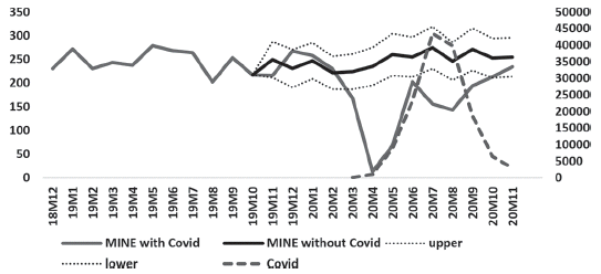
Figure 6: COVID-19’s impact on the mining sector Variations in COVID-19 cases are measured on the right axis.Source: Author’s elaboration based on data from INE and Bolivia Segura.
The sector initiated a V-shaped recovery up to June only to fall back again during the peak contagion months of July and August, and finally ending with a tilted W-shaped recovery. The November confidence interval suggests there might be no difference between the observed and counterfactual values, thus the sector might have been able to fully recover by that month. The width of the confidence intervals from November 2019 to February 2020 suggest no clear difference between the observed and counterfactual series, thus it is not possible to establish with accuracy how the November 2019 political conflict affected this sector and how fast it recovered from it. Computation of the accumulated difference establishes a dramatic loss of economic activity in the average order of -34.94% in magnitude in the period between February to November 2020, within a range from a worst scenario of a -44.1% loss to a best scenario of a -22.2% loss. By May, when the strict pandemic quarantine was ending, the sector had already accumulated an average of -49% loss of activity.
4.4. Manufacture industries
The monthly rhythm and evolution of economic activity in the Bolivian manufacturing sector is followed by the Manufacturing Industries index (MANUF for short). This sector has been growing at an annual average rate of 4.55% for the five-year period from 2015-2019, following an annual seasonality with the months from April to November of highest economic activity and in recent years particularly concentrated between August to October, and from January to March, the months of lowest economic activity, particularly February. How would the MANUF series have behaved if COVID-19 pandemic didn’t happen? Figure 7 is the result of the exercise where the MANUF with COVID line corresponds to the evolution of the manufacturing sector as it was observed and registered by INE and the MANUF without COVID line represents how the sector index would have behaved if neither the political conflict nor the pandemic had occurred or counterfactual, within dotted confidence intervals.
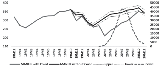
Figure 7: COVID-19’s impact on the manufacturing sector Variations in COVID-19 cases are measured on the right axis.Source: Author’s elaboration based on data from INE and Bolivia Segura.
The visual difference between both lines shows the significant magnitude of the pandemic’s impact on the manufacturing sector for the period of ten months between February and November 2020, but mostly concentrated on the whole period from April to October, and following a tilted reversed L-shape full recovery up to November. The observed difference in November 2019 is due to the impact of the political instability event on economic activity that month and from which the sector recovered quickly. Computation of the accumulated difference shows the sector experienced an average loss of economic activity in the order of -14.79% in magnitude (within a confidence interval from -18.30% to -10.96%), again in the period from February to November 2020. By May, when the strict pandemic quarantine was ending, the sector had already accumulated an average of -18.92% loss of economic activity.
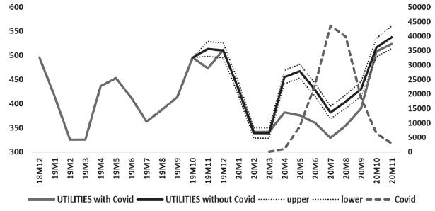
4.5. Electricity, gas and water
The monthly rhythm and evolution of economic activity in the Bolivian utilities sector is followed by the Electricity, Gas and Water index (UTILITIES for short). This sector has been growing at an annual average rate of 4.36% from 2015-2019, following an annual seasonality with April, May and particularly October to December, being the months of highest economic activity, while February, March and July the months of lowest economic activity. How would the UTILITES series have behaved if COVID-19 pandemic didn’t happen? Figure 8 is the result of the exercise where the UTILITIES with COVID line corresponds to the evolution of the utilities sector as it was observed and registered by INE and the UTILITIES without COVID line represents how the sector index would have behaved if neither the political nor the pandemic had occurred or counterfactual, within dotted confidence intervals. The visual difference between both lines shows the magnitude of the pandemic’s impact on this sector for the period of ten months between February and November 2020, mostly concentrated on the months from April to September, but managing a full recovery of its growth path by October and November. The observed difference in November 2019 represents the impact of the political instability event on economic activity that month from which the sector recovered immediately. Computation of the accumulated difference shows this sector experimented an accumulated average loss of economic activity of -9.12% (within a confidence interval from-12.12% to -5.89%) with August the month of highest accumulated loss of activity (-11.71%).
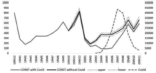
4.6. Construction industry
The monthly rhythm and evolution of economic activity in the Bolivian construction sector is followed by the Construction Industries index (CONST for short). This sector has been growing at an annual average rate of 4.73% for the five-year period from 2015-2019, following a clear annual seasonality with December the month of highest economic activity and February the month of lowest. How would the CONST series have behaved if COVID-19 pandemic didn’t happen? Figure 9 is the result of the exercise where the CONST with COVID line corresponds to the evolution of the construction as observed and registered by INE and the CONST without COVID line represents how the sector index would have behaved if neither the political conflict nor the pandemic had occurred or counterfactual, within dotted confidence intervals. The visual difference between the two lines shows the pandemic’s impact on this sector for the period of ten months between February to November 2020, mostly concentrated on the months from April to July, months were the sector was usually picking up, then from August to November the sector almost managed to reach its growth path level. Since the latter are months of high regular activity the sector was able to avoid greater economic loss. Earlier the sector was affected very little by the November 2019 political instability event. Computation of the accumulated difference shows this sector experimented a dramatic average loss of economic activity in the order of -34.49% in magnitude (within a confidence interval from -39.64% to -28.37%) in the period between February to November 2020, with June the month of highest accumulated loss of activity (-58.1%).
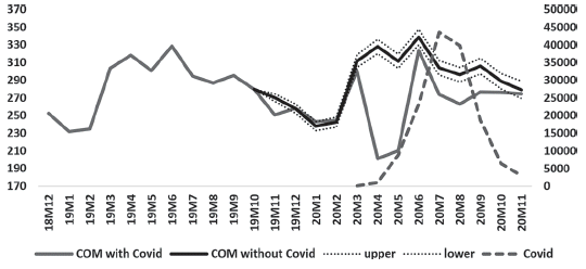
4.7. Commerce
The monthly rhythm and evolution of economic activity in the Bolivian commerce sector is followed by the Commerce index (COM for short). This sector has been growing at an annual average rate of 4.51% for 2015-2019 following an annual seasonality with the months from April to June of highest economic activity, particularly June, and with January and February, the months of lowest economic activity. How would the COM series have behaved if COVID-19 pandemic didn’t happen? Figure 10 is the result of the exercise where the COM with COVID line corresponds to the evolution of the commerce sector as it was observed and registered by INE, and the COM without COVID line represents how the sector index would have behaved if neither the political conflict nor the pandemic had occurred or counterfactual, within dotted confidence intervals. The visual difference between the two lines shows the pandemic’s impact on the commerce sector for the period of ten months between February and November 2020, but mostly concentrated on April and May, months that usually are of high economic activity. By June it almost fully recovered following a U-shape but the increase in COVID-19’s cases in July and August finally determined a W-Shape full recovery by November. The observed difference in November 2019 is due to the impact of the political instability event on the sector’s economic activity that month and from which it recovered quickly. Computation of the accumulated difference shows a sector that experimented an average loss of economic activity of -12.04% in magnitude (within a confidence interval from -14.36% to -9.59%) in the period between February to November 2020, with May the month of highest accumulated loss (-19.86%).
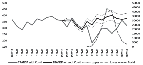
4.8. Transport
The monthly rhythm and evolution of economic activity in the transportation sector is followed by the Transport and Storage index (TRANSP for short). This sector has been growing on average at an annual rate of 4.48% for the five-year period from 2015-2019 following an annual seasonality of high economic activity from May to December with August its highest, and low economic activity from January to April with February its lowest. How would the TRANSP series have behaved if COVID-19 pandemic didn’t happen? Figure 11 is the result of the exercise where the TRANSP with COVID line corresponds to the evolution of the transport sector as it was observed and registered by INE, and the TRANSP without COVID line represents how the sector index would have behaved if neither the political conflict nor the pandemic had occurred or counterfactual, within dotted confidence intervals. The visual difference between the two lines shows the pandemic’s impact on the transport sector for the period of ten months between February and November 2020, but mostly concentrated on the period from March to September, months that usually are of high to the highest level economic activity. Some recovery began in June and July, however the increase in COVID-19’s cases in July and August finally determined a W-Shape recovery up to October. The observed difference in November 2019 is due to the impact of the political instability event on the sector’s economic activity and from which it recovered immediately. Computation of the accumulated difference shows this sector experimented an average loss of economic activity of -20.91% in magnitude (within a confidence interval from -27.47% to -13.04%) in the period between February to November 2020, with August the month of highest accumulated loss of activity of close to -25%.
4.9. Communications
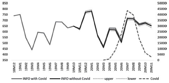
The monthly rhythm and evolution of economic activity in the communications sector is followed by the Communications index (INFO for short). This sector has been growing at an annual average rate of 4.26% for the five-year period from 2015-2019, following an annual seasonality with the months from July to January of high economic activity with January the highest, and low economic activity from February to June, with March the lowest. How would the INFO series have behaved if COVID-19 pandemic didn’t happen? Figure 12 is the result of the exercise where the INFO with COVID line corresponds to the evolution of the communications sector as it was observed and registered by INE, and the INFO without COVID line represents how the sector index would have behaved if neither the political conflict nor the pandemic had occurred or counterfactual, within dotted confidence intervals. The visual difference between the two lines shows the pandemic did not have a negative impact on this sector during the ten months first wave period from February to November 2020, but rather it might have benefited from it a bit during the months from April to June. In effect, when computing the accumulated difference there is an average gain in economic activity of +1.36% in magnitude (within a confidence interval from -0.31% to +3.08%). However, its confidence interval suggests no impact at all, although the interval has a bias towards the positive. In fact, June is the month of highest average accumulated economic gain (+2.20%). Also, the November 2019 political instability event didn’t have any impact on this sector.
4.10. Financial establishments, insurance and real state
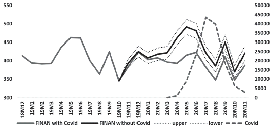
The monthly rhythm and evolution of economic activity in the financial sector is followed by the Financial Establishments, Insurance and Real Estate index (FINAN for short). This sector has been growing at an annual average rate of 5.68% from 2015-2019, following an annual seasonality of highest economic activity in May and June and lowest in August and October. How would the FINAN series have behaved if COVID-19 pandemic didn’t happen? Figure 13 is the result of the exercise where the FINAN with COVID line corresponds to the evolution of the finance sector as it was observed and registered by INE, and the FINAN without COVID line represents how the sector index would have behaved if neither the political conflict nor the pandemic had occurred or counterfactual, within dotted confidence intervals. The visual difference between the two lines shows the pandemic’s impact on the sector for the period of ten months between February and November 2020, but mostly concentrated on the months of April, May and June usually of highest economic activity. The sector did manage to recover its regular seasonal pattern from July to November, however just below its counterfactual level due to the July-August pandemic peaks. The November 2019 political instability event basically didn’t have an impact on this sector. The computed percent loss in economic activity reached an accumulated average of -9.53% (within a confidence interval from -13.23% to -5.49%) with monthly accumulated loses just above -10% from May to September.
4.11. Public administration services
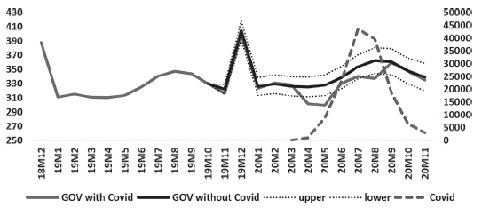
The monthly rhythm and evolution of economic activity in the public sector is followed by the Public Administration Services index (GOV for short). This sector has been growing at an annual average rate of 5.88% for the five-year period from 2015-2019, following an annual seasonality with December the month of highest economic activity and from January to April and November of lowest. How would the GOV series have behaved if COVID-19 pandemic didn’t happen? Figure 14 is the result of the exercise where the GOV with COVID line corresponds to the evolution of the government sector as it was observed and registered by INE, and the GOV without COVID line represents how the sector index would have behaved if neither the political conflict nor the pandemic had occurred or counterfactual, within dotted confidence intervals. The visual difference between the two lines shows the pandemic’s impact on this sector for the period from February to November 2020, mostly concentrated on the months from April to August which include months of usually low and high economic activity. However, not all of the monthly differences appear to be true departures from the counterfactual due to the width of the dotted confidence intervals. The months of April. May and August do show evidence of negative impacts from the pandemic. Forecast accuracy might be affected by the December extreme observation which the model does capture. Nevertheless, by September the sector fully reaches its counterfactual seasonal pattern and level following what appears a W-shape recovery. The November 2019 political instability event basically didn’t have an impact on this sector. The computed percent loss in economic activity shows the government sector experienced a small accumulated average of -2.93% (within a confidence interval from -7.31% to +1.88%) with August the month of highest accumulated loss (-4%). However, in the end the range of the confidence interval (mostly negative but containing zero) for this accumulated average suggests no impact, even though there is evidence of negative impact. In this case the pandemic’s impact on the Government sector cannot be determined.
4.12. Restaurant, hotels and community, social, personal and domestic services
The monthly rhythm and evolution of economic activity in the restaurants and hotels sector is followed by the Restaurant, Hotels and Other Community, Social, Personal and Domestic Services index (RHS for short). This sector has been growing at an annual average rate of 4.26% for the five-year period from 2015-2019 prior to the pandemic, following an annual seasonality with highest economic activity in December and January and low economic activity from February to April with March its lowest. How would the RHO series have behaved if COVID-19 pandemic didn’t happen? Figure 15 is the result of the exercise where the RHS with COVID line corresponds to the evolution of the RHO sector as it was observed and registered by INE, and the RHS without COVID line represents how the sector index would have behaved if neither the political conflict nor the pandemic had occurred or counterfactual, within dotted confidence intervals.

Figure 15: COVID-19’s impact on the restaurants & hotels sector Variations in COVID-19 cases are measured on the right axis.Source: Author’s elaboration based on data from INE and Bolivia Segura.
The visual difference between the two lines shows the pandemic’s impact on the restaurants and hotels sector for the period of ten months from February to November 2020, particularly hit between the eight months from April to November, with April, May and June the worst. Though it began with a U-shape recovery staring July, in the end it could not reach its counterfactual level not even by November. The observed drop and immediate recovery in November 2019 are due to the political instability event that month. When the average percent loss in economic activity is computed it shows this sector experienced an average accumulated economic loss in the order of -20.68% in magnitude (within a confidence interval from -21.55% to -19.80%), with accumulated monthly loses above -20% since May.
5. Summary and concluding thoughts
Table 2 is a summary of COVID’s impact on the Bolivian economy globally and by economic sectors. The difference between the observed and counterfactual time series produces an average global economic activity loss of -12.64% during the 10-month period from February to November (last row in the Table). This loss means it cannot be recovered or in other words Bolivians are either 12.64% poorer or less rich. Recovery means the degree at which the economy has reached the counterfactual level of production and growth path which would have happened if the economic crisis caused by the COVID-19 pandemic did not occur. The sooner the economy recovers the sooner the economy stops loosing economic wealth. The last column shows that by November the overall economy recovered on average 96.7% of its expected counterfactual level of activity for that month.
Table 2 Summary of COVID-19’s impact by economic sectors and overall IGAE
| Sector of economic activity | COVID-19's impact | Average degree of recovery by November |
|---|---|---|
| Communications | No impact (slight positive bias) | Highly resilient |
| Agriculture, livestock, forestry, hunting and fishing | No impact (slight negative bias) | Highly resilient |
| Electricity, gas and water | -9.12% (-12.12%,-5.89%) | Full |
| Financial establishments, insurance and real estate | -9.53% (-13.23%,-5.49%) | 92.1% |
| Commerce | -12.04% (-14.36%,-9.59%) | Full |
| Manufacture industry | -14.79% (-18.30%,-10.96%) | Full |
| Restaurants, hotels and communal, social, personal and domestic services | -20.68% (-21.55%,-19.80%) | 88.1% |
| Transport and storage | -20.91% (-27.47%,-13.04%) | 85.1% |
| Construction | -34.49% (-39.64%,-28.37%) | 88.1% |
| Metalic and non-metalic minerals | -34.94% (-44.10%,-22.20%) | Full |
| Public administration services | Undetermined | Full |
| Crude oil and natural gas | Undetermined | Undetermined |
| Overall IGAE |
-12.64% (-15.77%,-9.26%) |
96.7% |
Source: Own. 95% confidence interval in parenthesis.
The breakdown of COVID-19’s impact into the 12 economic sectors, also from February to November, shows that only the communications and agricultural sectors were not impacted by the pandemic but rather were highly resilient. While the rest simply lost, with minerals and construction the most damaged (-34.94% and -34.49%), followed by transportation and restaurants & hotels (-20.91% and -20.68%), manufacture industries and commerce (-14.79% and -12.04%), and finance and utilities (-9.53% and -9.12%). The pandemic’s impact on the oil & gas and government sectors could not be determined. However, at the same time, by the end of the first wave in November most sectors were able to recover fully or at levels above 85%. Full recovery in all sectors would have taken some short additional time, however that possibility did not happen due to the pandemic’s continuation with new waves beginning in December 2020 and going well into 2021 without a clear ending.
Recovery across sectors was heterogeneous in the sense that most sectors did not follow exactly the global tilted W-shape economic recovery within the 10-month period from February to November 2020, but rather followed different speeds, times and magnitudes affecting economic connections across sectors and the overall structure of the economy. These disconnections among sectors may become an important operating issue in a prolonged pandemic scenario, which will force its own adjustment and structural change. Also, the loss of “momentum” as firm’s investment projects are postponed further adds to lost time, activity, interconnections and output.
The question of how prepared was each sector to quickly change to its digital counterpart or how much digital adaptation was able to occur during the pandemic is probably important to understand the heterogeneous recovery. The decision of many to simply go out and work versus work from home either partially or fully digitized is also important to understand that heterogeneous recovery. The large Bolivian base of self-employed, micro and small enterprises are predominantly contact-intensive and they operate basically in all sectors of the economy, particularly in agriculture, commerce, transportation, construction, mining, oil & gas downstream, manufacturing, and restaurants & hotels. At the same time, most of the management and administrative staff from all sectors are currently operating either partially or fully digitized, as well as service sectors like utilities, communication & information services, finance, insurance & real estate services, and education services. Many more services within each sector could have their digital counterpart operating soon enough, particularly most government services.
The ability of the estimated models to produce short-term monthly counterfactual series works well for impact measurement and graphical analysis during the period of Covid’s first wave. However, the pandemic continues and several Covid waves are expected throughout 2021 and maybe even 2022. In this persistent pandemic scenario, measuring loss of economic activity by prolonging the counterfactual series would result in diminishing accuracy as their confidence intervals get increasingly wider. In this case an alternative would be to switch to lower frequency time series like the quarterly GDP, although at the cost of losing rich monthly data analysis2.
As in all crisis there are good and bad outcomes, certainly the loss of economic activity, which was this paper’s emphasis, qualifies as a bad one but the digital transformation it brought all over the economy and beyond qualifies as a good outcome for the present and the future. In some cases, it required the deepening and expansion of digitalization but, in most cases, it meant the introduction of digitalization, learning by doing and a slow initiation at the challenge of the economy’s digital transformation. In any case, the Bolivian economy was quite behind in the adoption, and much less so in the research & development, of the new digital technologies and the innovation possibilities they bring which ultimately are expressed in efficiency gains, transparency, its focus on people’s preferences and needs, new business models and customer experience, new government service models and citizen experience, the appearance of prosumers, and all the cultural changes it brings, in other words the expansion of economic, social, political and cultural freedoms, however not without its own particular problems like privacy and security concerns and more generally regulatory concerns as well as the potential widening of the digital divide at least in its initial stage.
Moving forward, in the short-run, despite individual efforts at adjusting our way of working and living and despite social efforts at adapting our economy to minimize the loss of economic activity under pandemic, the solution to the COVID-19 pandemic lies outside the economic sphere and Bolivia’s own efforts at tackling it, it also lies in the world’s management of the pandemic, the politics of cooperation among nations and surely COVID economics too. The worldwide new waves of the pandemic with new COVID-19 variants along with progress in the vaccination front, is still going on in 2021 within the natural world’s climate and seasons, and it might take an additional year or two to finally end the pandemic worldwide, however, all of its accumulated economic consequences may take much longer.
The long-term solution to the source of the problem, COVID-19 contagion, depends on how the Bolivian society tackles the issue, whether with a passive attitude of permanently waiting for the rescue from the international community and their vaccines or a proactive attitude by fully accepting the problem as an opportunity to enter into own research & development in the biological sciences with a long-term view connected to international research centers.

