ARTÍCULOS CIENTÍFICOS

 

Monetary dynamics in post inflation Bolivia

 

Dinámica monetaria en Bolivia después de la inflación

 

 

Jonathan Fortun-Vargas^*

 

 

---

Summary

Is inflation always explained as a monetary phenomenon?. In this study, the author presents empirical evidence regarding the relation of Money Growth and its effect on Inflation, for the specific case of Bolivia. The text describes the situation of the country analyzed in terms of monetary policy after one of the worst cases of hyperinflation ever; empirical evidence is presented trough two independent estimations, one following the Cochrane-Orcutt procedure, and the other following a Box-Jenkins procedure (ARMA process) that confirms the relation between Money Growth and Inflation in Bolivia using data for the years 1998 to 2010.

Keywords: Inflation; money growth; quantity theory of money; monetary policy; Latin America; Bolivia.

---

Resumen

¿Son los procesos inflacionarios siempre atribuibles a fenómenos monetarios?. En este estudio el autor presenta evidencia empírica de la relación entre crecimiento de la base monetaria y su efecto en la inflación, para el caso específico de Bolivia. El texto describe la situación del país analizado en términos de política monetaria luego de uno de los peores casos de hiperinflación; se presenta evidencia empírica a través de dos estimaciones independientes, una siguiendo un procedimiento Cochrane-Orcutt y la otra a través de un procedimiento Box-Jenkins (proceso ARMA), los cuales confirman la relación entre crecimiento de la cantidad de dinero e inflación en Bolivia, usando datos para los años 1998 a 2010.

Palabras clave: Inflación; crecimiento del dinero; teoría de la cantidad de dinero; política monetaria; Latinoamérica; Bolivia.

JEL Codification: E31, C32, E51, O23

---

 

 

1. Introduction

One of the most famous discussions in economics and specifically in macroeconomics is the continuing controversy and debate over the relationship between money growth and inflation. Despite this discussion, it is generally accepted that, historically, increases (decreases) in the trend growth rate of the money supplyhave been verystrongly associatedwith increases (decreases) in trend inflation¹.

The scheme where constant changes in the price level are associated with changes in the supply of money is one of the oldest and most established propositions in economics (Dwyer & Hafer, 1999). one of the first antecedents to this proposition is found on the almost 250 years-old David Hume’s essay "of Money", where the author analyzes the link between increases in money and the subsequent increase in prices (Hume, 1752). economists since this time have observed over and over that prolonged increases in prices are associated with increases in the nominal quantity of money.

Summarizing the findings, Milton friedman in 1963 coined the idea that "Inflation is always and everywhere a monetary phenomenon" (Friedman, 1994). In recent time the work of leading economists such as Mccandless & Weber (1995), Dwyer & Hafer (1988), Dewald (1998), Barro (2008) and many others have found that changes in the nominal quantity of money and the price level are closely related.

Regardless of the long and enduring evidence that suggest a correlation between money supply and inflation, this association is still disputed. One possible explanation for this disagreement according to Dwyer and Hafer is that the empirical relationship between money growth and inflation is present only over time periods that are so long that the relationship is uninformative for practitioners and policymakers, are more concerned about inflation next month or next year (Dwyer Jr & Hafer, 1988).

There exist several techniques to estimate the empirical evidence between Money Growth and Inflation, some of recent studies by Hallman, Porter, & Small (1991) explore the idea of a linear estimation, while Crowder (1998) Bokhari & Ferdun (2006), Capistrán & Ramos-Francia (2009) explore econometric techniques using autoregressive methods and error corrections.

Moreover, the discussion is broader when it deals with experiences in countries with distinctive features regarding its monetary history; such is the case of Bolivia.

The question that I try to assess in this study deals with the consequence and more importantly time lag that an expansion of the monetary base has on inflation. This question is especially interesting in the case of the Bolivian economy where there has been and still exists a high rate of dollarization (as it will be discussed later on this paper), therefore the question of the relation between the expansion of local currency against inflation in a highly dollarized country seems interesting.

1.1. The Latin American Case

A distinctive characteristic of developing countries in general, and Latin American countries in specific, is that money creation is an important source of government revenue (Harberger, 1978).

In recent times, inflation has been low worldwide, and Latin America is not an exception. in the 10 largest Latin American economies (Argentina, Bolivia, Brazil, Chile, Colombia, Ecuador, Mexico, Peru, Uruguay, and Venezuela), consumer price inflation went from a quarterly average of 24% in the 1980s to 15% in the 1990s and to 2% in the first 7 yr of the 2000s (Capistrán & Ramos-Francia, 2009).

A large number of countries in Latin America and worldwide have acquired the technique of inflation targeting as their preferred framework for monetary policymaking with the final goal of keeping inflation low and stable (De Mello & Moccero, 2009). Attainment of this policy objective depends crucially on the monetary authority’s ability to anchor inflation expectations around a preannounced target. In this sense, it has been argued that inflation targeting is really about targeting expected inflation (Svensson, 1999).

Despite the well understood and popular belief of the importance of documenting the dynamics of inflation, it seems that there has been almost no effort to understand the dynamics of inflation for Latin American countries (LAC). This is a very surprising fact for two reasons.

Firstly, the analysis of the dynamics, causes and effects of inflation in LAC can be very helpful to amplify our understanding of the inflation dynamics in general given the fact that LAC have had both more frequent and larger monetary regime switches than developed economies; LAC have experienced various rollercoaster inflation periods of low as well as high inflation and monetary regimes that cover, among many others, fixed and flexible exchange rates, hard pegging, currency boards, money targeting, and (as discussed before) recently inflation targeting. Moreover, the Latin American region has been hit by diverse shocks closely related to inflation, for example, the shocks of oil price, financial crises, continuous devaluations, Balance of Payment crises, etc.

Second, the lack of serious academic research characterizing the dynamics of inflation in LAC is even more surprising since some of these countries have made public their commitment to keep inflation low (after the rampant inflation and hyperinflation processes suffered in the region during the late 80s and early 90s), and a required condition to accomplish this objective seems to be an understanding of inflation and their relevance with the macroeconomic perspective of a country.

Latin American countries present numerous shifts in their inflation figures, far more numerous than in developed countries, moreover these shifts tend to occur in a synchronized manner (among LAC countries). A clear example of this is the inflation increasing throughout the eighties and then decreasing from the beginning of the nineties onward, with a few temporary upturns in some countries. Hence, the great inflation and the inflation stabilization in Latin America occurred with a lag compared with the developed countries. (Capistrán & Ramos-Francia, 2009)

 

2. Analytical Framework

2.1. The quantity theory of money

The quantity theory of money is typically used to explain the long-run determinants of the price level and the inflation rate. The quantity theory of money is originated in the work of early monetary theorists, including the work of David Hume, as stated before. In short, this theory states that money supply has a direct, proportional relationship with the price level.

The link between transactions and money is expressed in the quantity equation:

Where T represents the total number of transactions during some period of time, in other words, is the number of times in certain period of time that goods or services are exchanged for money. P is the price of a typical transaction, this product (TxP) must equal the number of monetary units exchanged in a given period of time, this portion of the equation deals with the transactions.

The LH of the equation explains the relation of money used to make the transactions. M is the quantity of money, V is the velocity of money, which measures the rate at which money circulates in the economy-the number of times a monetary unit changes hands in a given period.

In the last equation, there seems to be a difficulty on measuring the number of transactions T, therefore, to simplify the calculations, T is often replaced by Y (total output of the economy). transactions and output are related given the accepted fact that the more the economy produces, the more goods are bought and sold. Therefore we have:

In the case of the analysis of how money affects the economy, it is useful to express the quantity of money in terms of the total amount of goods and services it could buy. The amount M/P should be the real money balances. from this we could infer the money demand function, which shows the determinants of the quantity of real money balances that the public is holding, this representation is given by:

Where k is a constant of the proportion of money that the public is willing to hold for every unit of income. Equation 3 states that the quantity of real money balances demanded is proportional to real income.

Some authors define inflation as "too much money chasing too few goods" (Barro, 2008)/. This definition encapsulates relevant aspects of why money growth is related to inflation. However, for our purposes we will define inflation as "increases in the general level of prices"(Mankiw, 2010)MA, USA, WH Freeman Co. isbn:9781429259354 rather than in terms of why increases in the general price level occur.

The relation between the growth of money quantity and inflation is ultimately based on the relation between supply and demand for money. There are several types of measure of money, but for the purposes of this study, we will use M2 as a correct measure of money.

2.2.  The Supply of money

Given the former gold standard, changes in the global supply of commodities (in specific gold) affected the supply of money, it is widely accepted that in today’s globalized economy this is not true anymore. Current governments affect the nominal quantity of money trough policy actions, such as open market operations, the change in reserves or changing the central bank funding rates to banks.

2.3.  The demand for money

The demand for money is fundamental to understand the interaction and effect of money growth and the level of inflation. The public will hold money to acquire goods and services. As a byproduct, the demand of households and firms for real quantity of money will rise. if prices suffer an increase, the society will have a propensity to hold more money to buy the same amount of goods.

Given the fact that M is considered the nominal quantity of money and P is the price level (as described in equation 1), then the real quantity of money is M/P (equation 3). The price level is usually measured by general price indexes such as the consumer price index and gross domestic product deflator. In short, the real quantity of money will be the nominal quantity of money adjusted for inflation.

If we talk about demand for money we can see that the single most important factor affecting the demand of money is the real income. For higher income, there is more spending, and more spending increases the portion of money holding in the society.

The single most important factor that affects the demand for money is real income. A higher level of income is associated with more spending, and more spending is facilitated by holding more money. A proportional relationship between the real quantity of money demanded and real income is a convenient form of the dependence of demand for money on income. This relation is the same one described in equation 3.

2.4. The price level

The price level can't be fully explained only by using supply and demand for money. If we look at equation 3, we can summarize the relationship among the nominal quantity of money, the price level, and real income as well as all of the other factors that affect the demand for money represented by the variable k.

In equation 3, if we let Y to be constant and the factors reflected in k besides than real income were constant also, rewriting we have:

Equation 4 is very useful for explaining the relation of price level against its determinants, or if we consider that k^-1= V, we have:

Equation 5 is the same as equation 4 but considering money velocity

2.5. The empirical problem on measuring the effect of money supply and inflation

If real income were constant and other factors did not affect the demand for money or were constant, then there would be a proportional relationship between the price level and the nominal quantity of money relative to real income (Mullineaux, 1980). If the nominal quantity of money M changed, then P would change by the same proportion because k and Y were constant. The change in real income trough time has an effect in the demand for money; the determinants for real income though, are not related to supply or demand of money, especially in long periods.

As explained by the long term production function and the solow model, the major factors affecting the growth of real income over time are growth of resources available to produce goods and services and technological change. More money printing does not have a real effect on the creation of labor or real capital to produce goods and services or to affect significant technological change. Therefore, we can conclude that at least over longer periods of time, real income is an independent variable, without relation to the nominal quantity of money or the price level. Finally, we can say that, any change in real income has an effect over the price level; however, there seems to be proportional relationship between the price level and the nominal quantity of money (in relation to real income).

If there is a relatively unimportant variation in the demand of money for reasons other than real income, indicated by the variable k in equations (3) and (4), then we can conclude that equation (4) indicates that the price level and money relative to real income are proportionally and directly related. A close relationship between the price level and the nominal quantity of money relative to income is not "needed" to explain this phenomenon.

On the other hand, if a variation in the demand for money for reasons other than real income is substantially more important than variation in the money supply relative to real income, then this variation in the demand for money can result in no observable relationship between the price level and money relative to real income.

Changes in the general level of prices will be related with changes in money demand, -k in equations (3) and (4), and not money relative to real income. The significance of variation in the supply of money and the demand for money for explaining the price level is therefore a challenge to be measured at an empirical level.

2.6. The special case of Bolivia

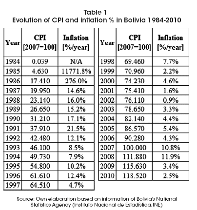
The inflation in Bolivia during 1984 and 1985 was the most rapid in Latin American history, and one of the highest in world history. During the twelve-month period, August 1984 to August 1985, prices rose by 20,000 percent, and during the final months of the hyperinflation, from May 1985 to August 1985, the inflation surged to an annualized rate of 60,000 percent (Sachs, 1986) 1986. The Bolivian inflation is the only case in thirty-five years of a "true" hyperinflation, applying Phillip cagan’s 1956 classic definition of price increases exceeding 50 percent per month².

After a great economical and social struggle, the Bolivian government with the help of world recognized economist Jeffrey Sachs formulated a financial program that curbed the hyperinflation. The program had a very basic premise: a balanced budget. Government spending shouldn't be more than its revenue. As the program began to work policy makers recommended that the Bolivian Central Bank use its funds to support the value of the Bolivian currency, and therefore a crawling peg system of exchange was created, called "bolsin" (Cariaga, 1996). Despite achieving the pursued goal of finishing hyperinflation, this policy had a contrary effect because it resulted in Bolivians who were afraid to hold their assets in Bolivian currency. The transfer of funds back into the Bolivian currency further shored up its value and led to even more capital outflows from the country.

Thereafter monetary and fiscal policy in Bolivia produced a relative stability, (see Table 1). However it did take more than a decade for the rate of inflation to reach levels consistently below 10% peryear.

Product of this set of policies and the tremendous trauma caused by the hyperinflation process, the Bolivian public showed a persistent loss of confidence in the national currency (boliviano), which caused a "de facto" dollarization process of the economy. To illustrate this point see Table 2, which compares the percentage of deposits in foreign currency for Latin American countries, the case of high dollarization in Bolivia is easily recognizable.

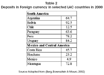
As stated in the introduction, this paper will assess the unique circumstances of the high dollarization on the Bolivian economy, and establish a relation between money growth and inflation for the recent post inflation era in Bolivia.

 

3. Data & Methodology

3.1. Data description

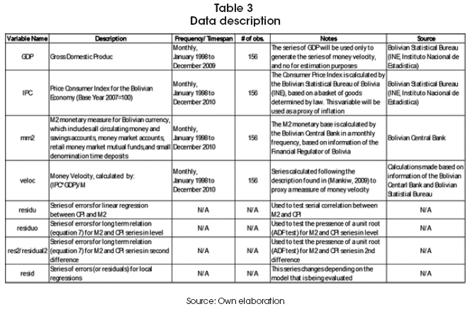
For the purpose of this study I will proxy the level of inflation by the CPI index calculated by the National Statistics Bureau of Bolivia (INE, Institution Nacional de Estadística). The monetary base M2 was retrieved from the Bolivian Central Bank (Banco Central de Bolivia), finally for illustrative purposes money velocity will be calculated using the data of GDP collected by the national statistics Bureau of Bolivia. for all the series the data has a monthly frequency. The data was collected between the years 1998 and 2010, the selection of this time frame is given by the fact that this research tries to evaluate the relation between inflation and money growth in a "post-hyperinflation" setting, and 1998 was the first year where Bolivia presented consistency in an inflation level below 10% (see table 11). It is important to note that for the regression the variables M2 and CPI will be transformed to log form to interpret and capture the effect of incidence in a more practical way.

Below I present a summary of the data for the series utilized in this research:

3.2. Methodology

To investigate the relation between inflation and money growth i will use two different approaches, the first one being a linear estimation, using the Cochrane-Orcutt estimation, the later using an ARMA model following a Box Jenkins specification and combining it with a Cochrane-Orcutt estimation. to summarize the methodology used in these two different approaches, refer to figure 1 and figure 2:

 

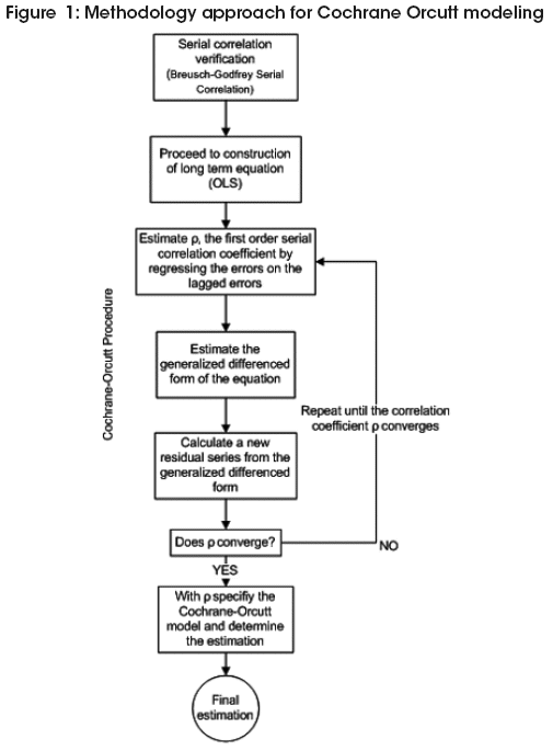
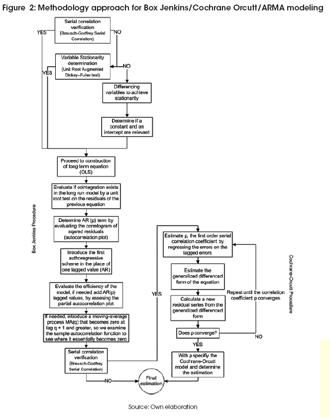
The next methodological approach selected combines the construction of an ARMA model, and after that correcting it trough a Cochrane-Orcutt procedure to achieve a healthier level without serial correlation.

As it can be seen on the previous figure, for both cases, the first step is to evaluate if there exists a serial correlation between the series, therefore I will first comment on the consequences of serial correlation:

3.3. The problems and consequences of serial correlation

When error terms from different (usually adjacent) time periods (or cross-section observations) are correlated, we say that the error term is serially correlated. Serial correlation occurs in time-series studies when the errors associated with a given time period carry over into future time periods. Serial correlation will not affect the unbiasedness or consistency of OLS estimators, but it does affect their efficiency With positive serial correlation, the OLS estimates of the standard errors will be smaller than the true standard errors. This will lead to the conclusion that the parameter estimates are more precise than they really are. There will be a tendency to reject the null hypothesis when it should not be rejected.

3.3.1. Testing for serial correlation

The most popular technique to test if serial correlation is present in time series is the Durbin Watson statistic³, defined by:

A Durbin Watson statistic will be defined in the 0-4 range, with a value near two indicating no first-order serial correlation. Values below 2 for this statistic are indication of positive serial correlation (whereas values above 2 indicate negative serial correlation)⁴, however several authors comment that the interpretation of the Durbin Watson statistic can be difficult (Pindyck & Rubinfeld, 1998). Therefore, for the purposes of this research, the Breusch-Godfrey test will be used to determine serial correlation in the series.

The Breusch-Godfrey test is a test to evaluate for autocorrelation in the errors. The null hypothesis is that there is no serial correlation of any order up to p.

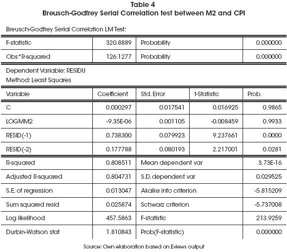
For the purposes of this study a Breusch-Godfrey test was rehearsed to test if serial correlation is present between the series in log form of M2 (money quantity) and CPI (price index, proxy of inflation), the details of this test can be reviewed on table 4 on the Appendix, where the confirmation of a Serial Correlation between the series is strong (the zero probability value strongly indicates the presence of serial correlation in the residuals).

3.4. Cochrane-Orcutt Procedure

To assess the relation between Inflation and Money Growth, I will firstly use a linear estimation using the methodology of the Cochrane-Orcutt procedure.

Cochrane-Orcutt estimation is a procedure in econometrics, which adjusts a linear model for serial correlation in the error term. As discussed in previous lines, a Breusch-Godfrey test confirmed the presence of serial correlation between Money Growth (M2) and Inflation (proxied by CPI).

It is important to note that despite the fact that in the following equations the variables ICP and M2 are used for illustrative ends, the natural log form for CPI and M2 is being used. in other words, in the following equations log(ICP)=ICP and log(M2)=M2.

Once the serial correlation is found, I proceed to construct the long term equation, by following classical specifications found in several papers such as (Bokhari & Ferdun, 2006; Capistrán & Ramos-Francia, 2009; Crowder, 1998):

Where ICP_t is the time series of consumer Price index (inflation) at time t, M2_t is the quantity of money at a given time in the economy (measured with the M2 monetary index) and _t is the error term. As discussed before the error term is serially correlated:

The Cochrane-Orcutt procedure will transform the model to:

Where the sum of squared residuals ε²_t is minimizedwith respect to the estimators (α,β) conditioned to ρ.

In practice, the Cochrane-Orcutt method is a multi-step procedure that requires re-estimation until the value for the estimated first order serial correlation coefficient (ρ) converges.

To compute the serial correlation coefficient, based on the errors of equation, rho will be computed by regressing the errors on the lagged errors as shown in equation. The serial correlation coefficient obtained in this step will not be the final rho coefficient, because -as explained before- there needs to be a re-estimation until convergence of the value is obtained. Once we obtain a (not real) rho value, I estimate a generalized differenced form (equation 9). After that, a new residual series _t must be calculated.

This must be repeated until convergence is found in the correlation coefficient, graphically:

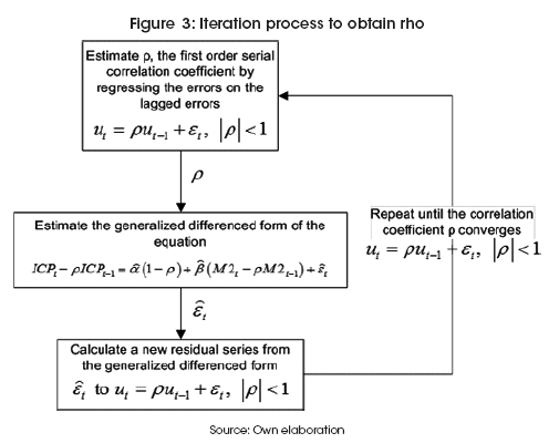
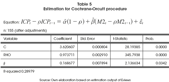
Once rho is determined (in this case after 4 iterations), the generalized differenced form of the equation is determined trough the Cochrane-Orcutt procedure, estimating the final values for the estimators, which can be found in the Annex on table 5.

3.5. Box Jenkins/ARMA estimation

The second approach to the estimation of the effect of Money Growth on Inflation will be trough the building of an ARMA model following the Box Jenkins procedure; before commenting on the specific procedure followed, it is important to give some commentary on which is the methodological base to use this approach:

3.5.1. Evaluation the long run relation of Money Growth and Inflation

If we rewrite equation considering that Y can be represented as the product of price and quantity (P*Q), and we suppose a linear price level, then we have:

Where k is the inverse of base velocity. If real output and real base money are both non-stationary and cointegrated, base velocity will be a mean reverting series. Figure 4 is a plot of the natural logarithm of base velocity. By evaluating the figure, it can be clearly seen that there is no evidence that the series reverts to a constant mean⁵.

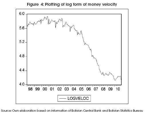
This discovery implies that the real monetary base and real income are not cointegrated⁶. This conclusion can also be suspected by looking at the linear representation of both series in Figure 5. The order of integration of GDP is not clear; however it is not the aim of this study to address this issue.

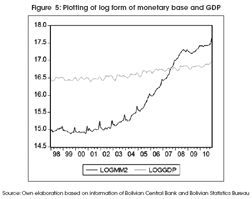
The above mentioned conclusions support the idea of performing an analysis of Linear Time Series by an ARMA estimation.

To understand the model, let’s suppose that there are y₁,y₂ ,...,y_t observations. Different from classical regression models, this model will not use a set of explanatory variables for modeling the relations between the variables. instead, the variable y is explained by relating it to its own past and historic values and also relating it to a weighted sum of current and lagged random disturbances.

The Autoregressive Moving Average (ARMA) (p,q) is represented by:

The variance, covariance and autocorrelation are solutions to difference equations

q is the memory of the moving average part of the time series so that for k≥ q+1 the autocorrelation function (and covariance) exhibit the properties of a purely autoregressive process. If the time series is homogeneous stationary, then after differenced the series y_t to produce stationary series w_t, there is the possibility to model w_t as an ARMA process.

3.6. The Box Jenkins procedure

In this methodological approach, I will use the Box Jenkins procedure for the construction of the ARMA model, with two slight differences from the classical approach: i) before checking for cointegration for every single series I will perform a test of serial correlation as in the previous approach, and ii) after obtaining the ARMA process if serial correlation is still found, I will perform a fixing of this problem trough the Cochrane-Orcutt procedure.

As previously established by the Breusch-Godfrey, serial correlation is present between the series in log form⁷ of M2 (money quantity) and CPI (price index, proxy of inflation)⁸.

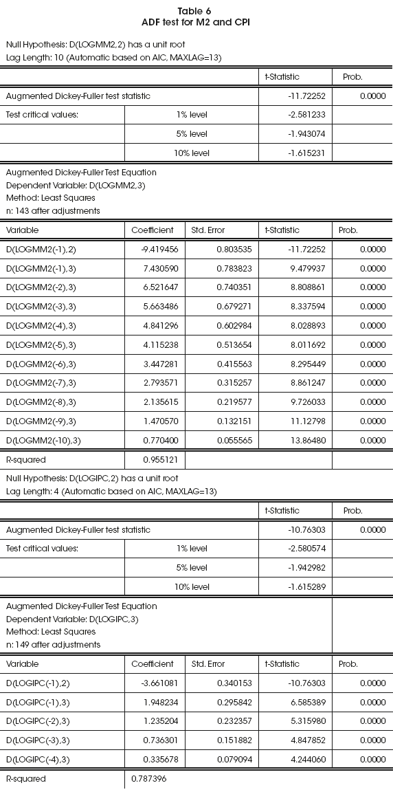
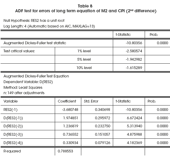
Despite the above finding, i will still check for the level of cointegration of the series M2 and CPI trough an ADf test⁹. The results of such tests can be found in the Annex in Table 6. As it can be seen, both, M2 and CPI are I(2) variables without a constant or intercept.

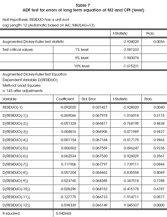
The next step on this process is to estimate a classic model as in equation and evaluate if cointegration exists in this model by a unit root test (ADf) on the residuals of this estimation.

It is important to note that from this point, and for consistency ends, the Box Jenkins procedure will be applied to the variables M2 and CPI on level (because of the serial correlation test) and as I(2) variables, thus creating two parallel procedures.

The unit root test for the residuals on the level for of M2 and CPI can be found in the Annex in Table 7, in the same way the same test for the I(2) variables of M2 and CPI is located in Table 8. The unit root test for the variables in level form reject the hypotheses that there is a unit root in the series (even at 1% level of confidence), the same expected result is given for the variables in second difference.

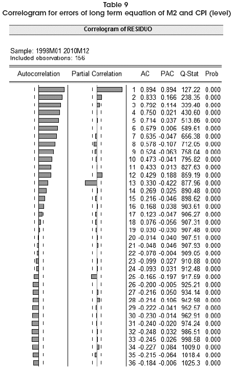
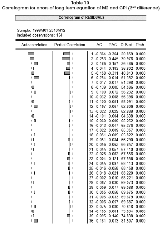
This allows us to continue to the next step on the estimation which deals with the determination of the AR(p) term by evaluating the correlogram of the squared residuals¹⁰ (once again this procedure will be rehearsed for the estimation with variables in level and second difference form).

Specifically for an AR(1) process, the sample autocorrelation function should have an exponentially decreasing appearance (Pankrátz, 1983) as shown in Table 9. Based on this fact, an AR(1) term will be introduced in the equation for the case of level series, whereas for the case of series in second difference an AR(1) term will be omitted since the correlogram for this specification (Table 10) does not present such behavior.

For higher-order autoregressive processes, the sample autocorrelation needs to be supplemented with a partial autocorrelation plot. The partial autocorrelation of an AR(p) process becomes zero at lag p +1 and greater, so we examine the sample partial autocorrelation function to see if there is evidence of a departure from zero (Brockwell & Davis, 2009). On the other hand, the autocorrelation function of a MA(q) process becomes zero at lag q + 1 and greater (Brockwell & Davis, 2009), sowe examine the sample autocorrelation function to see where it essentially becomes zero.

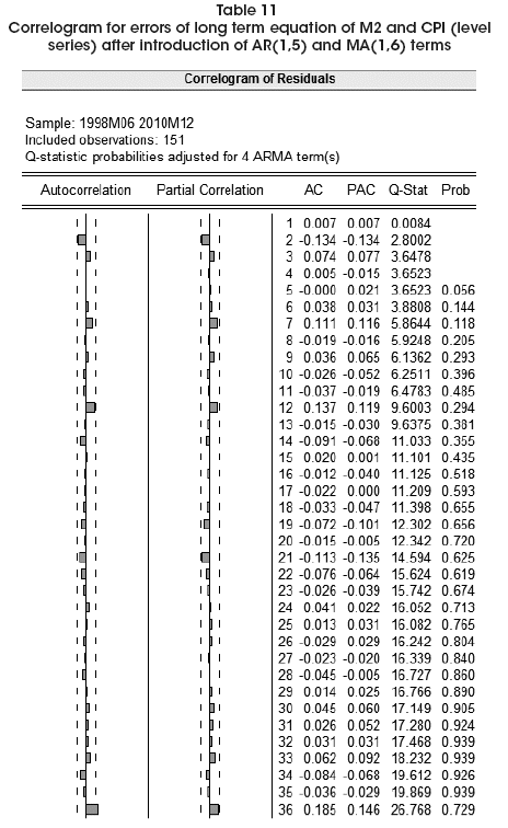
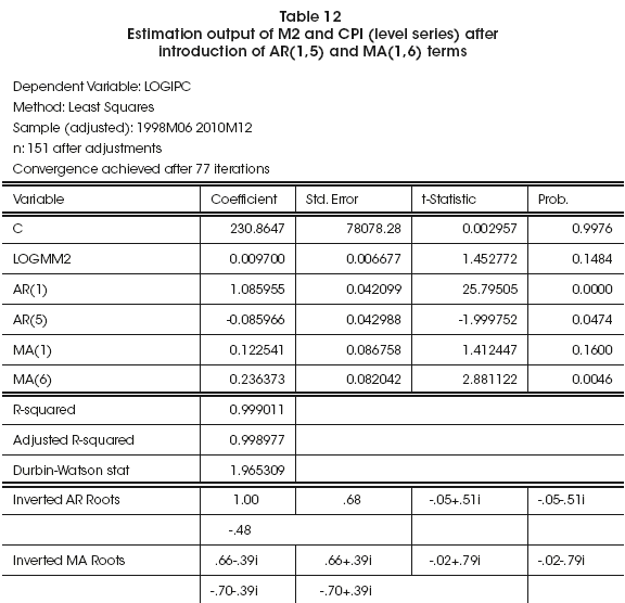
Following this criteria we add AR(p) and MA(q) terms until the sample autocorrelation function becomes zero in a certain point¹¹ (confirm the presence of white noise)¹². for the model in level variables, this stage is achieved at a AR(1,5) MA(1,6) model. However with this model specification, the significance level for the M2 series is too low (measured by its t-statistic), which presents us with the situation of "spurious inference" (all the symptoms of such problem exist, such as the presence of a very high R², low significance level of the regressor, etc.)¹³ therefore the model specification with level variables is dropped.

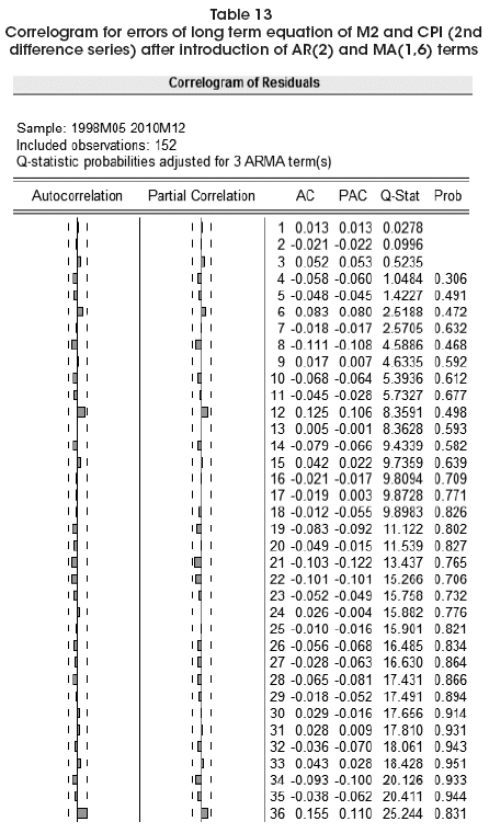
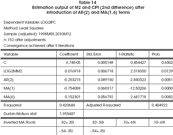
On the other hand, when working with the model specification with variables in second difference, white noise is found with a specification of AR(2) MA(1,6). Moreover when we evaluate the t statistics in the terms of the estimation we can see that all of them are significant¹⁴. This specification becomes our short term equation and final ARMA specification.

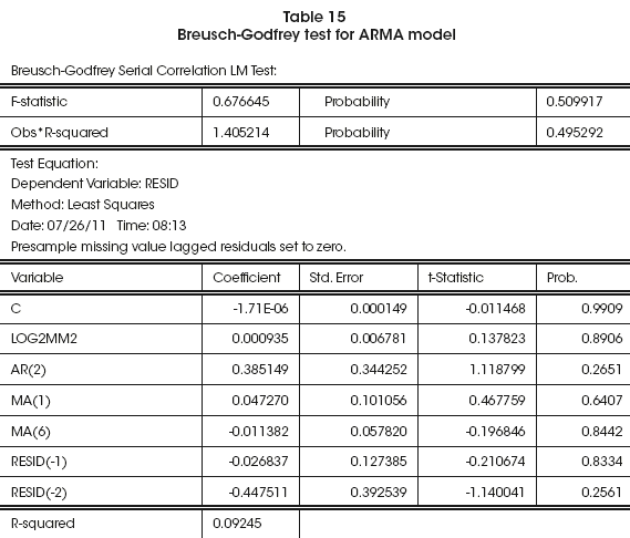
At this point we have arrived to the end of the Box Jenkins methodology for identification of ARMA specified models (the statistical significance and economic interpretation of such model will be addressed on the next section). However as an additional step in this specific research, this final ARMA estimation will be evaluated for serial correlation trough a Breusch-Godfreytest¹⁵.

After performing the test, it is easy noticeable that serial correlation is not present on the residuals (the above zero probability of nearly 51% strongly indicates the absence of serial correlation in the residuals). It is important to note thatwe can arrive to the same conclusion by evaluating the Durbin Watson statistic from the ARMA estimation¹⁶.

By confirming the absence of serial correlation on the residuals of the ARMA specification, this becomes our final model.

 

4. Results & discussion

For this section, i will present the results and conclusions for the two independent processes, trying to link them to an explanation of the economic phenomenon that is taking place.

4.1. Cochrane-Orcutt process

The estimation output for the model estimation including rho is in the Annex in Table 5. From this output we can determine that there is a relation between inflation and money growth after correcting the model for serial correlation¹⁷.

Leaving other variables constant, the expansion of the local currency monetary base in Bolivia, explains 16% of the increment on inflation measured by the Consumer Price Index. This result is in line with several studies that link inflation and money growth in the long run -such as (Bokhari & Ferdun, 2006; De Mello & Moccero, 2009; Dwyer & Hafer, 1999; Mullineaux, 1980)-, however the level of incidence is fair lower than in the studies cited previously, this result could be explained by the high level of dollarization in Bolivia. Also, given the circumstances of the exchange system in Bolivia (a crawling peg), the control over money growth has beentight, leaving little space to have an active monetary policy in the country.

Despite the value of the coefficient the relation between inflation and money growth is confirmed, even for a highly dollarized country such as Bolivia. This country has a very unique structure where most of the time the general population has a preference for foreign currency rather than local currency, despite this fact, the finding that money growth has an important incidence on inflation was expected. We should also analyze the exporting structure of Bolivia, where commodities dominate the spectrum, this reality added to the low efficiency and competitiveness of the country, pushes the central Bank and monetary authorities to constantly devaluate the local currency to support exports, which ultimately has an effect on the monetary base, and as shown here, a transmission to inflation. Moreover, and not landing too far away from the previous comment, even though being mainly a commodities producer, Bolivia imports some first necessity goods such as sugar and flour, which have an important incidence on inflation given the recent price elevation of commodities.

As clear as this result is, it is important to note that a linear estimation does not asses two important facts when dealing with inflation, this technique can't identify the time (number of periods) that this effect of money growth on inflation has. This information is very important when trying to understand the dynamics of an economic phenomenon such as inflation. Moreover, the conclusion that the incidence is low can't be taken as an absolute true given the fact that the expansion of the monetary base has several spillover effects that are not assessed in this estimation.

4.2. Box Jenkins process

In short the AR(p) process will explain that the level of the current observation depends on the level of its lagged observations (autoregressive part), while the MA(q) process represents the fact that the observations of a random variable at time t are not only affected by the shock at time t, but also the shocks that have taken place before time t (moving average part).

As it can be already suspected, this process solves the two problems cited in the cochrane-Orcutt process.

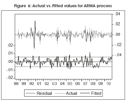
The final estimation for this model can be found in the Annex in Table 14. If we assess the econometric reliability of the model we can comment that the estimated results are similar to the actual values if we look at figure 6 in the Annex. The inverted roots of the characteristic polynomial (z) = 1 + 0.2532z - 0.754z² - 0.1523Z³ are complex and have modulus inside the complex unit circle¹⁸ so that the fitted model is stationary and ergodic¹⁹.

The plot of the actual, fitted and residuals indicate that the model tracks the simulated data well. The correlogram of the residuals (Table 13) reveals no omitted serial correlation AR(2) MA(1,6).

 

5. Conclusion

Talking about the economic significance of the model, it can be seen that the AR(2) process explains that the level of current inflation depends on the level of the money quantity of two past periods (months) on average, while the MA(1,6) process represents the fact that the observation of the inflation level in any given random time inside the sample is not only affected by the shock at that time, but also the shocks of monetary expansion that have taken place 1 and 6 months before respectively.

This conclusion shows the complex but interesting dynamics of inflation in Bolivia. Money growth has a confirmed incidence in the level of inflation at any given time. Moreover it is noticeable that the expansion of the monetary base has two different repercussions in the inflation, one in a short period of time within one month of the expansion and the other trough a semester. This result is somehow expected given the time and several control factors of inflationary process that a crawling peg system has in a country such as Bolivia. It can also be argued that the first shock is given for the great relevance and attention that the general population has on the monetary base (because of the historic reasons cited above), additionally the second later shock can be explained by the fact that the Bolivian economy is highly dollarized but at the same time the main monetary actors in Bolivia (the central Bank and 13 commercial banks) have a very control over the money quantity given to the general population, nevertheless, this finding is important and could be used to formulate better policies regarding the monetary policy makingin Bolivia and LAC .

It is interesting to note that the level of inflation highly depends on the level of money quantity two months before; again this effect can be explained by the restrictions and controls of the central Bank on the access of general population to new money. Moreover, it is also important to note that the operations inside the stock exchange in Bolivia are almost insignificant for the general population, aspect that supports the idea of a control of banks and financial institutions of the monetary base at least for the first part of a monetary expansion, this effect could also have some incidence on the rate of money velocity presented in the country.

The findings here are in line with previous studies of (Ball & Sheridan, 2003; Capistrán & Ramos-Francia, 2009; Dwyer & Hafer, 1999; Hofstetter, 2009; Mullineaux, 1980; Svensson, 1999), however to the understanding of the author this is the first experience rehearsed with a data set in a post inflation setting in Bolivia.

Despite the rigorous treatment of the data, a test for endogeneity of the series was not performed; this seems to be the biggest place where future studies could improve the present one (in an econometric technique way). On the same aspect, further work on this topic could be made regarding the inclusion of other variables that interact directly (or indirectly) with the level of inflation, such as the deposits level in banks or world prices of commodities. Moreover, the slow publication of new data by the Bolivian institutions makes further research of the interaction with other variables somehow complicated.

Finally, in a policy wise perspective, the findings of this research are important to firstly understand the dynamics of inflation in Bolivia and second tune up the incipient monetary policy on the basis of the fact that given the right kind information, policymakers could be able to apply shock policies in the short term to expand (or contract) the amount of money in the economy and at the same time smooth the (negative) impact that such policy could have over inflation.

 

Artículo recibido: 2 de noviembre de 2011
Manejado por: ABCE
Aceptado: 15 de abril de 2012

 

Appendix

All the tables and graphs are constructed by the author, based on estimations and information provided by econometric software.

 

 

 

 

 

 

 

 

 

 

 

 

Notas

* Graduate School of International Cooperation Studies, Kobe University, Kobe, Japan.
Contact. fortun@stu.kobe-u.ac.jp

1 (Grauwe & Polan, 2001) argue trough empirical evidence that the existence of a long-run relationship between money growth and inflation should be revised. (Nelson, 2003), on the other hand, challenges the results of Grauwe and Polan.

2 To expand in Cagan's definition see Cagan (1956).

3 For a detailed explanation in the Durbin Watson statistic, see Durbin & Watson (1950)

4 As a rough rule of thumb, if Durbin-Watson is less than 1.0, there may be cause for alarm. Small values of DW indicate successive error terms are, on average, close in value to one another, or positively correlated. If DW>2 successive error terms are, on average, much different in value to one another, i.e., negatively correlated. In regressions, this can imply an underestimation of the level of statistical significance (Brockwell & Davis, 2009)

5 This deduction is confirmed by an ADF test performed on the series, which cannot reject the null of a unit AR root in levels, this result represents a robust result to lag length (constant) and inclusion of a time trend.

6 This conclusion is confirmed when performing a Johansen cointegration test (as trace or max Eigenvalue) on the variables of M2 and GDP at level.

7 As stated before, throughout this procedure, the log form for M2 and CPI will be used, therefore in any equation M2=log(M2) and CPI=log(CPI)

8 The details of this test can be reviewed on Table 4 on the Appendix, where the confirmation of a Serial Correlation between the series is strong (the zero probability value strongly indicates the presence of serial correlation in the residuals)

9 The ADF test (augmented Dickey-Fuller test) is a test for the existence of a unit root in a time series sample. The ADF statistic is a negative number. As more negative it is, as stronger the rejection of the hypothesis that there is a unit root in the series.

10 The correlogram for the level form can be found in Table 9 and for the second differenced variables in Table 10.

11 This is usually determined by placing a 95% confidence interval on the sample partial autocorrelation plot (in other words a Probability value greater than 5% in the test of autocorrelation).

12 It is important to note that while the procedure tries to find white noise trough the insertion of AR(p) MA(q) processes, the significance of the original dependent variable (in this case M2) shouldn`t be too low (measured by its`t statistic), otherwise there is a risk of the presence of a "spurious inference" problem described in Granger & Newbold (1974).

13 The final correlogram for the model with level series can be found on Table 11 and its estimation on Table 12, where the high value for R2 and low significance of the variable M2 can be clearly notice.

14 The final correlogram for the model with series in second difference can be found on Table 13 and its estimation on Table 14.

15 Results of the Breusch-Godfrey test for the final ARMA model can be found on the Annex on Table 15.

16 A DW statistic of 2 or nearly 2 (in this case 1.9654) indicates no autocorrelation.

17 It is important to say that the value obtained for rho (after the iteration process) in this specification (Table 5) should have the same coefficient of an AR(1) term if we add it to the original equation (not shown here, but verifled), however an estimation such as this does not present an optimal shape of the autocorrelation function of the errors.Therefore, and to avoid this problem the Box Jenkins procedure is performed.

18 The complex unit circle is defined as the set of complex numbers that have norm (or modulus) equal to 1 (Hamilton, 1994)

19 Ergodic systems have the property that, given sufficient time, they include or impinge on all points in a given space and can be represented statistically by a reasonably large selection of points (Brockwell & Davis, 2009)

 

References

1. Ball, L. & Sheridan, N. (2003). Does Inflation targeting Matter?. NBER Working Paper No.9577.

2. Barro, R. J. (2008). Macroeconomics: A Modern Approach South-Western Pub.

3. Berg, A.; Borensztein, E. & Mauro, P. (2002). An evaluation of monetary regime options for Latin America* 1. The North American Journal of Economics and Finance, 13(3), 213-235.

4. Bokhari, S. M.H. & Ferdun, M. (2006). forecasting Inflation through econometric Models:An empirical study on Pakistani Data. Do u Üniversitesi Dergisi, 7(1),39-47.        [ Links ]

5. Brockwell, P. J. & Davis, r. A. (2009). Time series: theory and methods. Berlin, Germany: Springer Verlag.        [ Links ]

6. Cagan, P. (1956). The monetary dynamics of hyperinflation. Studies in the quantity theory of money (pp. 25-117). chicago, USA: University of Chicago Press.

7. Capistrán, C., & Ramos-Francia, M. (2009). Inflation Dynamics in Latin America. Contemporary Economic Policy, 27(3), 349-362        [ Links ]

8. Cariaga, J. L. (1996). Estabilización y desarrollo: importantes lecciones del programa económico de Bolivia. La Paz, Bolivia: Editorial Los Amigos del Libro.        [ Links ]

9. Crowder, W. J. (1998). The long run link between Money Growth and Inflation. Economic Inquiry, 36(2), 229-243.        [ Links ]

10. De Mello, L. & Moccero, D. (2009). Monetary Policy and Inflation expectations in Latin America: Long-Run Effects and Volatility Spillovers. Journal of Money, Credit and Banking, 41 (8), 1671-1690.        [ Links ]

11. Dewald, W.G. (1998). Money still matters, review. Federal Reserve Bank of St. Louis, 80,13-24.        [ Links ]

12. Durbin, J. & Watson, G. S. (1950). Testing for serial correlation in least squares regression: I. Biometrika, 37,409-428.

13. Dwyer, G. &Hafer, R. (1999). Are money growth and inflation still related?. Economic Review (Q2), 32-43.        [ Links ]

14. Dwyer Jr, G. P. & Hafer, R. W. (1988). Is money irrelevant? Federal Reserve Bank of St. Louis Review, 70(3), 3-17.        [ Links ]

15. Friedman, M. (1994). Money mischief: Episodes in monetary history. Mariner Books.

16. Granger, C. W.J. & Newbold, P. (1974). Spurious regressions in econometrics. Journal of Econometrics, 2,111-120.        [ Links ]

17. Grauwe, P. D. & Polan, M. (2001). Is Inflation Always and everywhere a Monetary Phenomenon? International Economics Working Papers Series.

18. Hallman, J. J._; Porter, R. D. & Small, D. H. (1991). Is the price level tied to the M2 monetary aggregate in the long run? The American Economic Review, 841-858.

19. Hamilton, J. D. (1994). Time series analysis. Boston, MA, USA: Princeton university Press.        [ Links ]

20. Harberger,A. C. (1978). A primer on inflation. Journal of Money, Credit and Banking, 10(4), 505-521.        [ Links ]

21. Hofstetter, M. (2009). Inflation targeting in Latin America: Toward a Monetary union? Documentos CEDE.

22. Hume, D. (1752). Of money. Essays, london: George routledge and sons.        [ Links ]

23. Mankiw, N. G. (2010). Macroeconomics. Boston, MA, USA: WH freeman & Co.        [ Links ]

24. Mccandless, G. T. & Weber, W. E. (1995). Some monetary facts. Federal Reserve Bank of Minneapolis Quarterly Review, 19(3), 2-11.        [ Links ]

25. Mullineaux, D. J. (1980). Inflation expectations and money growth in the united states. The American Economic Review, 70(1), 149-161.        [ Links ]

26. Nelson, E. (2003). The future of monetary aggregates in monetary policy analysis* 1. Journal of Monetary Economics, 50(5), 1029-1059.

27. Pankrátz, A. (1983). Forecasting with univariate Box-Jenkins models: concepts and cases. Chicago, USA: Wiley & Sons.        [ Links ]

28. Pindyck, R. S. & Rubinfeld, D. L. (1998). Econometric models and economic forecasts. Boston, MA, USA: Irwin/McGraw-Hill.

29. Sachs, J. D. (1986). The Bolivian hyperinflation and stabilization. National Bureau of Economic Research Cambridge, Mass., USA. AEA Papers and Proceedings, 77(2) May 1987

30. Svensson, L.E.O. (1999). Inflation targeting: some extensions. Scandinavian Journal of Economics, 101 (3), 337-361.        [ Links ]