The Dynamics of Poverty in Bolivia

 

 

Alejandro F. Mercado*, Jorge G.M. Leiton-Quiroga**

 

 

---

Abstract

The research aims to the understanding of the main factors that explain the dynamics of poverty in Bolivia. A main working hypothesis is that poverty is strongly linked to low social mobility levels. Social mobility can be defined as the equality of opportunities, or in other words, the probability that somebody can reach a better social position independently of his position of origin.

We rely in the concept that low social mobility generates a vicious poverty circle in which households that were poor yesterday, will see that their children are poor today, and with high probability, their children's children will be poor tomorrow. Indeed, our research hypothesis is that the dynamics of the phenomenon (the vicious circle) is explained fundamentally by two self reinforcing factors - ethnic and gender discrimination; which in turn lower the social mobility levels in a dynamic framework. This is proved partially along this research, especially for the subsets of indigenous women.

---

Resumen

La presente investigación tiene como objetivo identificar los principales factores que explican la dinámica de la pobreza en Bolivia. La hipótesis de partida es que la pobreza está ligada a una baja movilidad social. La movilidad social puede ser definida como la igualdad de oportunidades, es decir, la probabilidad de que los individuos puedan mejorar su posición social independientemente de su posición de origen.

Consideramos que la baja movilidad social genera un círculo vicioso de pobreza en el cual los hogares que fueron pobres ayer son pobres hoy, y, con alta probabilidad, los hogares de sus hijos también serán pobres. Nuestra hipótesis es que la reproducción de la pobreza se explica, en gran medida, por dos factores: la discriminación étnica y la discriminación por género, elementos que actúan profundizando la baja movilidad social.

---

 

 

Introduction

Poverty in Bolivia has become an endemic phenomenon, and the country has achieved strong support from international donors in order to fight poverty. More than 60 per cent of the total population is poor in Bolivia, and more than 80 per cent of total rural population is poor. In this regards, our research tries to understand the dynamics of poverty throughout the analysis of the Social Mobility Index by population subsets. One of the leading approaches in the study of the dynamics of poverty in Bolivia was proposed by Mercado (1992). In this study the author argues that the high rate of global participation of members of a household in the labor market penalizes the children's educational attainment. The low earnings of the parents pressure children to exchange school hours for working hours in order to meet the minimum income requirements of the household. Later on, this translates into a worsened laborers conditions (in terms of skills), and lower income levels, which reinforces child labor in the future. This generates a vicious circle where children leave school today, worsening their working opportunities for the future and worsening their ability to keep their children in school in the future.

In the late 1990s the interest to study the causes and the dynamics of poverty focused on the problems of the education system. The methodology proposed by Altonji and Blank (1999) was used to study the phenomenon in Bolivia. The central elements of these investigations referred to the quality of education and the ethnic and gender discrimination.

The work of Dahan and Gaviria (2000) and Andersen (2001) constituted the background to study poverty in Bolivia from the viewpoint of social mobility. Andersen (2003) and Mercado et al. (2005b) concluded that low social mobility is caused by the low quality of public education, and this becomes one of the main factors that explain the dynamics of poverty.

Therefore, according the previous investigations and their findings, we follow this research with the assumption that the main factor that explains the dynamics of poverty in Bolivia is linked to low social mobility levels. We mean by social mobility: the equality of opportunities, that is to say, the probability that somebody can reach a better social position independently of his or her position at origin. Low social mobility generates a vicious poverty circle, in which households that were poor yesterday, will see that their children are poor today, and with high probability, their children's children will be poor tomorrow (Mercado, et al., 2002).

Although, low social mobility in Bolivia is closely related to ethnic discrimination, we have some evidence that this phenomenon is reinforced by gender discrimination. And this is the core concept around which the present research aims to give some answers.

Therefore, our research hypothesis acknowledges the fact that social mobility is one of the main factors that explains the dynamics of the poverty circle in Bolivia. Indeed, our research hypothesis is that the dynamics of the phenomenon (the vicious circle) is explained fundamentally by two self reinforcing factors -ethnic and gender discrimination; which in turn lower social mobility levels in a dynamic framework.

Our research will analyze ethnic discrimination, contrasting the social mobility levels within sub samples: i) indigenous vs. non-indigenous; ii) male vs. female; iii) and a crossed analysis combining i. and ii. results. In summary, the objective of this research is to extend our knowledge on the causes that explain the dynamics of poverty in Bolivia. For this, we will try to identify the main variables that explain the low levels of social mobility. We will start with the hypothesis that low social mobility is explained by high levels of ethnic and gender discrimination.

Section 2 provides a brief background regarding poverty in Bolivia and its link with social mobility. Section 3 explains the methodology used in the research. Section 4 provides the results and empirical evidence. Finally the concluding remarks are at the end of the paper.

 

1. The Bolivian Context

The Bolivian economic growth for the period of 1952 to 2006 showed a modest behavior; on average, the economy rate of growth was very close to the population's rate of growth (Mercado. et al. 2002). Poverty in Bolivia has become an endemic phenomenon, we were poor yesterday, we are poor today and, most likely, we will be poor tomorrow. Bolivia has experimented with almost all conceivable economic policies. We have nationalized, privatized, capitalized and nationalized again, while we continue to be stuck in poverty.

Alongside the public economic policies, increased public expenditures only resulted in larger fiscal deficits, devaluations did not have a noticeable effect on our balance of payments, on the contrary, they only imposed disincentives to the national productive apparatus by raising the prices of imported capital goods, and an expansive monetary policy only resulted in a reduction of net international reserves and a reduction in the purchasing power of the local currency due to inflationary pressures. We opened up the economy to the free trade and, in other periods, we closed the economy, however all the efforts were vain, the economy stayed in much reduced levels of growth.

The actual poverty status in Bolivia is very high, indee'd, the country maintains the higher poverty levels in the South America. But beyond the actual poverty numbers' we want to highlight the concept that a poverty rate of fifty per cent poverty can mean two completely different things. One interpretation of this might be that the probability of becoming a poor person is 50 per cent; or from another point of view, the whole population is poor half of the time. That means that the 50 per cent of the population is always poor, while the remainder is unlikely to become poor. If the same households are poor all the time, it is much more difficult to develop strategies to alleviate the hardship. Poor people cannot save for harder times, as all times are hard, and they cannot borrow against higher future income because they don't expect their incomes to be any better in the future. It seems that the best strategy is to transfer knowledge and skills to this deprived population in order to prepare them to enhance their entitlements management in the future².

In accordance with a study carried out by the Institute of Socio-Economic Research (IISEC) of the Bolivian Catholic University (Mercado et al., 2005), the tendency factors are more important than the short run factors to explain economic growth, that means that the structural restrictions are more important than those linked to the economic policies, and these structural constraints reduced the economic policies effect in the short run. This idea is supported by Klasen et al. (2002), who highlights the strong dichotomy among the behavior of urban economic agents versus their rural counterparts. The production function is not consistent between them in terms of technology, production scale, workers skills and most importantly products. This situation constitutes a restraint of the Bolivian economic growth from this lack of technological progress of rural areas.

This diagnosis has led to the investigators to examine about the structural factors that would be restraining the economic growth. Andersen (2003) introduced within the explanatory variables the low social mobility index, she demonstrated the high correlation between the low social mobility index and the low rate of growth for the Bolivian economy. Other investigations, such as Mercado et al. (2005), corroborated Andersen's initial discoveries, at the same time they demonstrated the little effectiveness that would have the economic policies in a context of strong structural restrictions.

Later works were focused to determine the factors that would explain the low social mobility, as well as to find the links between the social sphere and the economic growth. The investigations of Mercado et al. (2004) and Leiton (2005) put their emphasis in the educational system, the segmentation in the social structure and the discrimination associated to factors of ethnic origin and gender.

We understand as social mobility the set of opportunities that the individuals have to ascend in the social scale, low social mobility implies that people are stuck somewhere in the income distribution scale year after year, and generation after generation. If the structural social factors -basically those referred to the household's heritable aspects-are important; then, the possibilities of social ascent are reduced, i.e. there exists a low social mobility condition. This implies the lack of a link between the efforts of people to overcome poverty such as training (studying several years), working harder, saving and investing; as they don't expect these efforts to pay off in the future and create a vicious circle, in which a low social mobility condition is reducing the incentives for growth, implying lower economic growth rates and which is reinforced in the next period by a low social mobility index, and so on (Vicious Circle of Poverty). In sum, when these efforts produce no payback, people make less effort and less incentives to growth, thus, the country doesn't growth.

The actual literature show us that the education is the most important factor concerning the social mobility, however, there other factors or barriers to social mobility, like the differences in education quality and education geographical scope between rich and poor people, even with public (free) education, there are still indirect costs: clothing, school supplies, transport, etc., and opportunity costs: due to low households' income levels, children are linked to domestic and farm work. The latter has became an important source of income for poor people.

Furthermore, the discrimination in the labor market reduces the returns to education to those population underprivileged segments. Extensive investigations have tried to account for discrimination and social group within the whole population. Mercado et al. (2004) have found that the marriage market corresponds to high levels of discrimination and that the structure of the marriage market imposes a discrimination strategy per se within social groups.

 

2. Methodology

The ISM will be calculated following the methodology proposed by Andersen (2003)³. In first instance the Fields Decomposition is applied to the results of the regression of the form:

Where:

X_t,i : Educational gap for period t and cohort i.

α : Constant term

β : Matrix of coefficients for the households' characteristics

Z_t,i : Matrix of households' characteristics

ε : Error term

We have defined the educational gap as the children's years old versus the number of years of education he has received at the moment of the survey, minus six years (which determines the time when children enroll the school).

However, the SMI is calculated based in a regression where the dependent variable is the educational gap and the explanatory variables are the "family records", for example, the level of the parents' education, the household's income, the parents' ethnic condition among others. If those variables are statistically significant to explain the educational gap, we conclude that the social mobility is low. The estimation through the Fields' decomposition will be applied to test the importance of each explanatory variable, through the relative contributions to the factorial inequality.

In order to answer the questions proposed in this research we have identified the following cohorts that will help us to understand the poverty dynamics in Bolivia. The Social Mobility Index is calculated for the periods 1993 and 2003-2004 with the Bolivian households' survey data. The periods proposed give us 10 years time span.

Also, we have taken into account people between 12 and 18 years old for the first cohort; between 19 and 25 years old for the second cohort and finally the total sample of 12 to 25 years old for the third cohort. Furthermore, we make distinction by gender and ethnicity characteristics. Therefore we obtain the following Social Mobility Indexes (See Table 1)

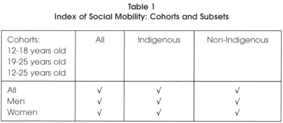
As the SMI is based on the educational gap, we only consider people that are between 12 to 25 years old. We expect that the results will show us no changes in the social mobility index between 1993 and 2003-2004. Also it is expected that the social mobility index is smaller for the indigenous women sub sample.

In the second step, and in order to identify the phenomenon in more detail, the above results allow us to calculate the variations of the SMI between the periods selected. In this regards, we will be able to acknowledge how people have evolved in terms of social mobility.

We expect that the SMI index will be lower in the crossed Indigenous-Women box Also, it is expected that the SMI is lower in the cases where the proportion of people that attend public schools is higher to those that attend private schools. As before, it is expected that the social mobility has not changed between 1993 and 2003-2004.

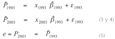
In the third step we will try to see the process from a more dynamic angle⁴. Thus, for the year 1993 we will take the same sub sample as before. Importantly, both age and education will be included within the educational gap. The same will be applied to the 2003-2004 survey and its subsequent estimations. Hence, with the previous results we follow the same methodology as in the SMI and contrast both results. How the differences help to explain the phenomenon? The estimation of the probability for a person to be poor in 1993 and remain poor in 2003-2004 leads us to important remarks about the permanent characteristics of poverty.

A poor-poor condition for both 1993 and 2003-2004 can show us the stickiness of poverty according specific characteristics; mainly making distinction by gender and ethnicity. According the explanation given above, we define the following econometric process in order to understand the phenomenon⁵.

Let.

P: The estimated educational gap

β: Model coefficients

ε: Statistical errors of all the regressions built for the SMI.

To examine changes in poverty over time (the dynamic effects) the following null hypothesis will be used:

If we cannot reject the null hypothesis then we conclude that the poverty circle is a permanent phenomenon. Rejection of the null hypothesis implies a transitory phenomenon. Or in other words, we can split our hypothesis according the following:

Where:

a)  Indicates a systematic behavior of poverty

b)  Indicates a permanent incidence of poverty

 

3. Empirical Evidence

This chapter starts the explanation with the identification of poverty in Bolivia, and subsequently we follow the analysis around the Social Mobility Index and Educational Gaps as explanatory variables of the dynamics of poverty in Bolivia.

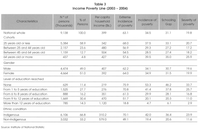
In order to characterize poverty within the country, let's take a look to Table 1, we can find the levels of poverty in Bolivia from 1999 to 2003. According the data, poverty incidence accounts for 63 per cent of total population, where indigenous people are more deprived with 70 per cent of poverty incidence. In the same table, we can highlight that indigenous people are more affected by extreme poverty⁶. Consistently, this replicates for urban areas, capital cities and for rural areas. The latter ones shows a deeper poverty condition, with more of 80 per cent of poverty incidence for indigenous people.

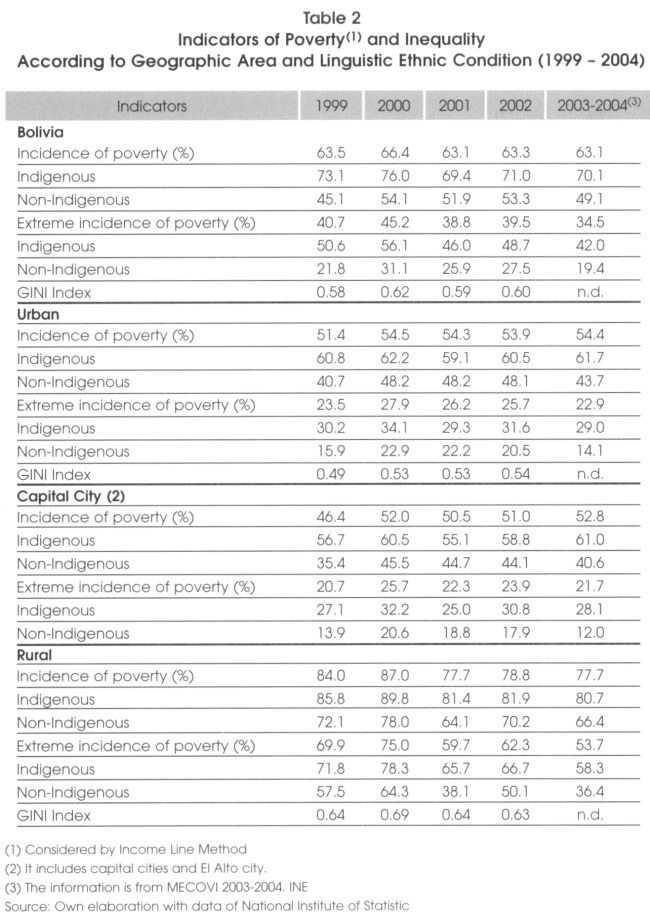
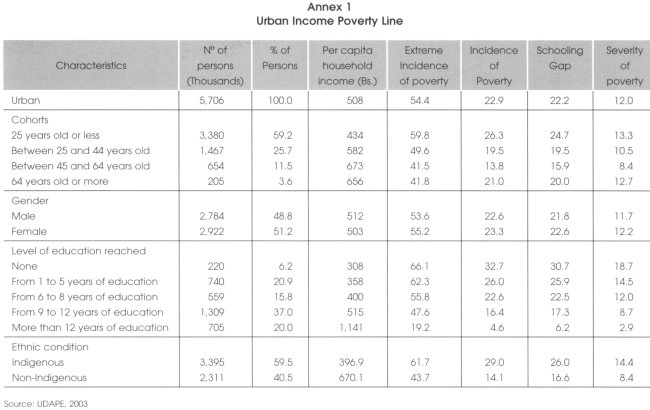
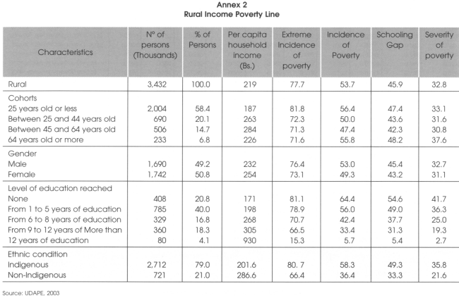
Furthermore, when we follow the analysis by gender situation, it is important to note that women are facing higher rates of poverty incidence rather than males. Table 3 shows us that phenomenon and also is possible to follow the analysis of poverty incidence throughout the number of years of education. Interestingly, as higher are the numbers of years of education, the poverty incidence ratio decreases consistently in all the cases⁷.

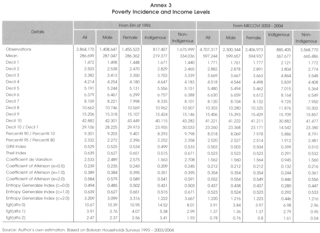
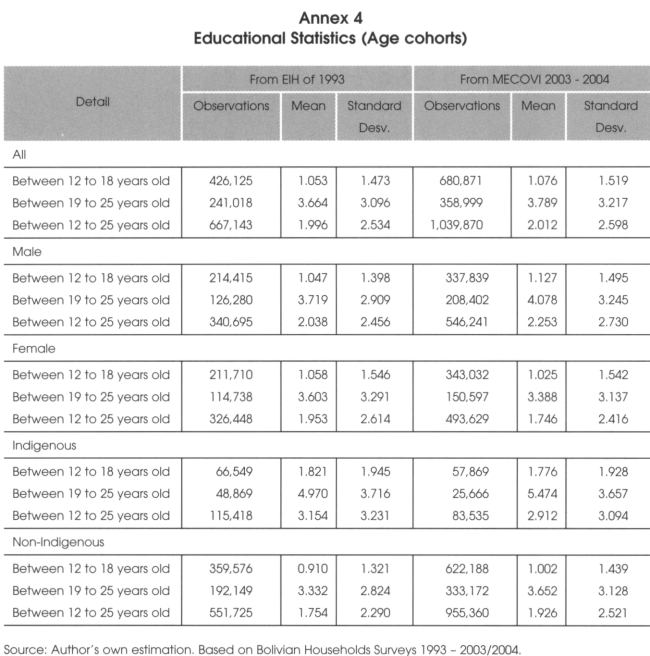
The households' income surveys that we have analyzed provides us results for poverty incidence in absolute numbers. The results are consistent with Table 2 and Table 3 explained above. Also, when we provide results (absolute numbers) for the average years of educations. Annex 3 and Annex 4 accounts for those results.

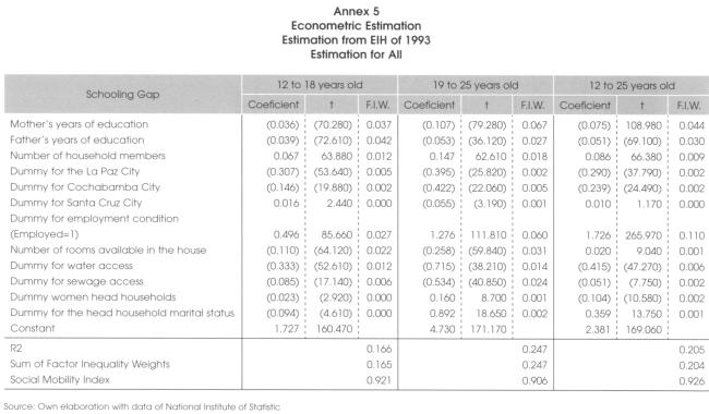
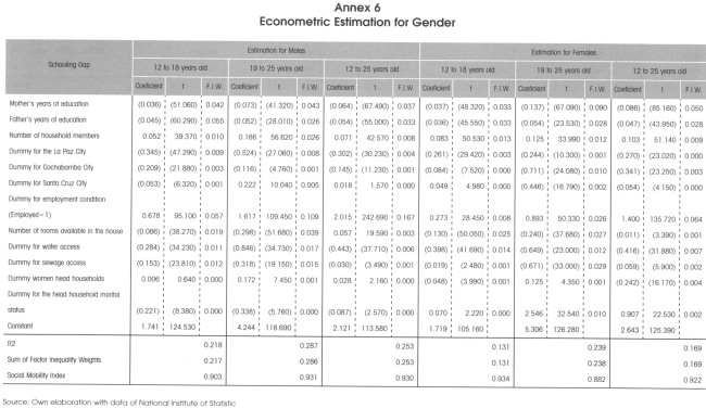
According the characteristics explained in the methodology, we have made the econometric estimation of the regressions (with the Ordinary Least Squares Method) for the calculation of the SMI and we have obtained the results showed in Annex 5 to Annex 14. The households characteristics included in the regression are:

Dependent Variable:

(10) SG: Education Gap = Years old - Years of education - 6

Explanatory Factors:

AEDUMA:        Mother's years of education

AEDUPA:         Father's years of education

MIEMBROS:  Number of household members.

REG2:             Dummy for the La Paz City

REG3:             Dummy for Cochabamba City

REG7:             Dummy for Santa Cruz City

OCUPADO:      Dummy for employment condition. Employed = I

DORMI:           Number of rooms available in the house

DAGUA:           Dummy for water access

DCLOACAS:     Dummy for sewage access

DJEFEMU:       Dummy women head households

DJEFESOL:      Dummy for the head household marital status

It is important to highlight that even though we follow the methodology proposed by Andersen (2003), we are not including the same explanatory variables due to the purposes of this research and also important to data constraints. Indeed, the data from early surveys such as the 1993s cannot provide more detailed information and we cannot follow the same households and persons in both surveys. Instead of, we are comparing the conditions for similar groups in two times in the space.

As we are studying only one country, the results of the SMI can differ from other studies, the comparisons made in previous studies are not the aim of this one. We are focused to acknowledge the behavior of the SMI within Bolivia. However, the SMI calculated by Andersen (2003) for Bolivia is 88 percentage points. We must keep in mind this feature at the time to interpret the results on Strategy Papers framework.

Table 4 show us the results for the first cohort studied, i.e. people between 12 and 18 years old and for all the subsets defined above. The results provide a very interesting performance of the SMI within the population subsets and within the time span selected. In terms of the full sample, the SMI has increased importantly and across the subsets this is reinforced steadily.

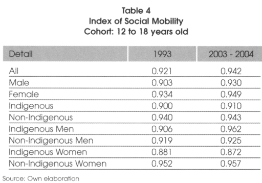
Now, what have happened with the male-female condition? Is it true that females are 'SMI worse-off rather than males?. The results shows mixed results, for the general women subset the SMI is higher than the males one. However, when we analyze the indigenous-women condition, the results points to a worsened SMI position; as was expected, indigenous women present the lowest SMI.

Furthermore, if we compare in general the indigenous condition versus the non-indigenous one, the result shows that the indigenous condition got a lower SMI rather than the non-indigenous.

Hence, we can rely in the assumption that those within the ethnicity condition are tied to lower education levels and lower access to development opportunities. From one point of view this can constitute a problem to overcome poverty and from another point of view, this can be understood as a structural barrier to further development (economic, political and social), which in turn need to be focalized and work towards its improvement.

Following our study, if we cross the analysis between indigenous condition and gender condition, again the results shows a worse off position for the indigenous women. Moreover, interestingly in 1993 non-indigenous people were better off rather their counterparts, but this is no true for the 2003-2004 results; we must highlight that the SMI shows a higher level of social mobility for the indigenous-males. These results presumably belong to the second generation reforms carried out in Bolivia during the 1990s. The governmental policies introduced by mid-1990s should have achieved important effects in terms of social development and access to opportunities and also, improvements in the effective use of entitlements (Sen, 1999). Within these policies we can highlight the most important ones: the educational reform, health system improvements, the new social security network reform, government decentralization (Participacion Popular), and all the social policies carried out within the Poverty Reduction Strategy Papers framework.

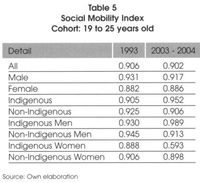
If we replicate the analysis for the next cohort (19-25) we find different results (See Table 5). In general, the SMI has not changed through time, and the conditions for people within this cohort are the same from the last 10 to 15 years. When we try to understand what is happening inside each subset we find several ups and downs in the index: aj as far as males presents the higher social mobility indexes in 1 993, this is not consistent with the results for 2003-2004. In the latter years there have been changes in the distribution of the index, with a lowered SMI for males in general; b) thus, as long as non-indigenous condition has lowered their SMI, the indigenous one has increased:

the same applies to indigenous males versus non-indigenous males; c) Also, for the women subset, the non-indigenous ones have maintained their SMI (at the limit), but for the indigenous women the situation has got worst. The indigenous women SMI have dropped by almost 30 percentages.

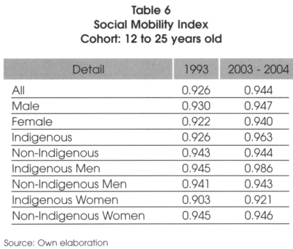
Finally, we need to observe what have happened in the full sample. For people between 12 and 25 years old, the results showed similar to the previous cohort. Again the women indigenous condition is the most disadvantaged one (see Table 6).

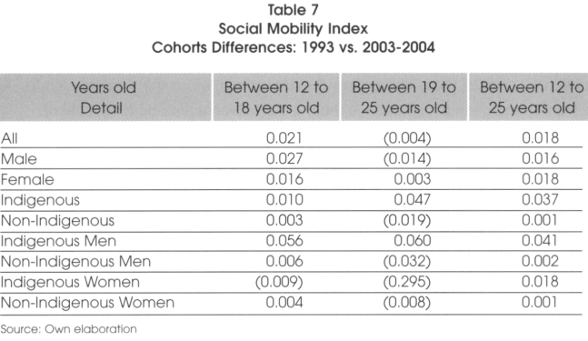
Consequently, we have made an exercise of SMI differences between the two periods proposed.

Table 7 provides us with the results with the following remarks:

•     In general, the SMI have shown a positive behavior (and almost zero for the 19-25 cohort)

•     People within the 19-25 years old did not benefit from the upward behavior of the SMI. In contrast, within this cohort, the index has experienced a downward trend for the following subsets: males, non-indigenous, non-indigenous males, and more heavily for indigenous women.

•     The most important improvements in the SMI were accounting within the 12-18 cohort, again proving the focus pointed by the Bolivian governments in poverty alleviation schemes alongside with the Poverty Reduction Strategy Papers.

•     The increments in the SMI seem to favor the indigenous conditions. The higher improvements are given in these subsets, except for indigenous women.

 

Now that we have acknowledged the patterns of the SMI by cohort and controlling by indigenous and gender conditions, we follow our methodology and we apply the criteria proposed in equations 2 to 5. Precisely, Table 8 provides us the results for equation 5⁸. We need to remember that we are now trying to understand the patterns of the educational gap inside the sub-sample used to study the Social Mobility phenomenon.

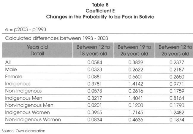
We have found an overall increase in the educational gap. Which is mainly explained by a higher increase for indigenous people, and specifically (and markedly) for indigenous women. These results are consistent with the ones explained above in the sense that, even though that indigenous people (males) are improving their education levels, it seems that the indigenous condition per se may represent a constrain to close the gap. This reinforces the idea that the earnings in terms of years of education ending with a higher social mobility index is greatly explained by the focused social programs implemented in Bolivia during the 1990s. Which has not achieved a sustainability status.

In general, the results shows that Bolivia as a hole has not reversed the widening educational gap and still is a binding problem to account for and overcome. This means that the economic conditions and the efforts that have been made in order to overcome poverty are not enough in this process. Even thought we have claimed that the social policies constituted an important pillar in order to overcome poverty and that have transferred better skills to the population that allow them to do a better use of their entitlements, the detailed results have mixed trends.

 

4. Final remarks

The poverty status in Bolivia has not changed dramatically along the last 15 years. The Social Mobility index has shown improvements in various segments of the population, but still there are important groups that are lagging behind.

For the 12-18 years old cohort and in terms of the full sample, the Social Mobility Index (SMI) has proved and increase, which replicates for the all the subsets males versus females, indigenous versus non-indigenous and the crossed analysis for the indigenous-gender condition.

In particular, the results are mixed for the women subsets. For the general women subset the SMI is higher than the males one. But, when we follow the analysis for the women indigenous, the results are disappointing due to a worsened SMI position. This proves our hypothesis about indigenous women with the lowest Social Mobility Index.

However, regarding the comparison between indigenous versus non-indigenous subsets, the results point to a better position of the non-indigenous population. Thus, in 1993 non-indigenous people were better off than the indigenous ones rather their counterparts, but unexpectedly, this is no true for the 2003-2004 results.

The governmental policies introduced by mid-1990s should have achieved important effects in terms of social development and access to opportunities and also, improvements in the effective use of entitlements.

For the 19-25 years old cohort, the SMI has not changed through time, and the conditions for people within this cohort are the same as for the last 15 years. But, we acknowledge that in the latter years there have been changes in the distribution of the index, with a lowered SMI for males in general; regarding the indigenous conditions there were observed an improvement of the SMI for the indigenous population, and a decrease for the non-indigenous segment. Also, for the women subset, the non-indigenous women have not presented a change. But the situation of the indigenous women has deteriorated to a great extent. Lastly, for the full sample (12-25 cohort), again the women indigenous condition is the most underprivileged.

Finally, we want to highlight the importance of social programs that seemed to got important effects in poverty alleviation levels. According the results obtained, the educative reform alongside the second generation reforms in Bolivia have introduced interesting steps towards poverty reduction. Low social mobility generates a vicious poverty circle, in which households that were poor yesterday will see that their children are poor today, and with high probability, their children's children will be poor tomorrow.

 

Notes

* Alejandro F. Mercado is Director of the Institute for Socio-Economic Research (IISEC - UCB)

** Jorge G.M. Leiton-Quiroga is Associate Researcher of the IISEC.

1    Incidence of poverty and extreme incidence of poverty in 2004 was 63.1% and 34.5% respectively.

2   We are taking the concept of entitlement as Sen (1999).

3 For a full description of Andersen (2003) methodology, please see appendix.

4   According the characteristics of the households' databases, we cannot use panel data estimation. The methodologies of each survey have changed. However we can perform other standard econometric analysis.

5   This methodology follows the one provided by Juhn et al. (1993).

6 Poverty incidence equals the head count ratio. Also extreme poverty is explained by 1 US$ poverty line per day.

7 Annex 1 and Annex 2 provides results for Urban and Rural scenarios

8 The estimation of equations 2 to 7 are provided in full in Annex 2

 

REFERENCES

Altonji, G. J. and R. M. Blank. 1999. "Race and Gender in the Labor Marker En O. Ashenfelter y D. Card (eds.) Handbook of Labor Economics 3c: 3143-3259.

Andersen. Lykke. 2003. "Baja movilidad social en Bolivia". Revista Latinoamericana de Desarrollo Económico. Septiembre. Universidad Catolica Boliviana. La Paz.

Dahan, M. and A. Gaviria. 2000. "Sibling Correlations and Social Mobility in Latin America" Interamerican Development Bank. Office of the Chief Economist. Draft. Marzo.

Fields, G.S. 1996. "Accounting for Differences in Income Inequality". School of Industrial and Labor Relations, Cornell University. Draft. Enero.

lnstituto Nacional de Estadistica. Encuestas de Hogares 1993. 2003, 2004. La Paz, Bolivia.

Juhn, Chinhui, Kevin M. Murphy and Brooks Pierce. 1993. "Wage Inequality and the Rise in Returns to Skill". The Journal of Political Economy, Vol 101, No. 3, June Pages 410-442.

Klasen, Stephany, Melanie Grosse, Rainer Thiele, Jann Lay, Julius Spatz and Manfred Wiebelt. 2002 Operationalizing Pro-Poor Growth. Country Case Study: Bolivia. KfW Entwicklungsbank (KfW Development Bank).

Leiton, Jorge G.M. 2005. "¿Existe una tendencia hacia la feminización de la pobreza?". Revista Latinoamericana de Desarrollo Económico. Abril. Universidad Católica Boliviana. La Paz.

Mercado, Alejandro F. 1 992. "Elementos para el diseño de políticas en el ámbito laboral". Fundacion Milenio. Mimeo. La Paz, Bolivia.

Mercado, Alejandro F, Lykke Andersen, Osvaldo Nina and Mauricio Medinacelli. 2002. "Movilidad social: clave para el desarrollo". Programa de Investigación Estratégica en Bolivia (PIEB) - lnstituto de Investigaciones Socio Económicas (IISEC) Universidad Católica Boliviana. La Paz.

Mercado, Alejandro F., Jorge G.M. Leiton and Fernando Rios. 2004. "Segmentación en el mercado matrimonial". Revista Latinoamericana de Desarrollo Económico. Octubre. Universidad Católica Boliviana. La Paz.

Mercado, Alejandro F, Jorge G. M. Leiton and Marcelo F. Chacon. 2005. "El crecimiento económico en Bolivia (1952-2003)". Revista Latinoamericana de Desarrollo Económico. Edición Especial, Julio. Universidad Católica Boliviana. La Paz.

Mood, A.M., FA. Graybill and D.C. Boes. 1974. Introduction to the Theory of Statistics. Third Edition, McGraw-Hill

Sen, Amartya. 1999. Development as Freedom. Oxford University Press.

 

 

 

 

 

Appendix A

Methodology

We provide a theoretical derivation of the Fields' Decomposition and thereafter we exemplify the calculus of the Social Mobility Index.¹

A.1 The Fields' Decomposition

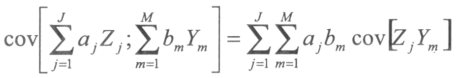
Let's define an income generating function of the form:

Where:

Y: logarithmic vector of individual's income within the sample

Z: defined as a matrix with j explicative variables, including the constant, education years, experience, squared experience, gender, etc., for each individual in the sample.

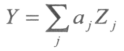
The income's log-variance is a simple inequality measure. Therefore, the variance is taken from both sides of the income function. The right-hand side can be modified with the following theorem:

Theorem (Mood, Graybill and Boes, 1974): Let Z₁.......Z_j ; and Y₁,.......,Y_M; two sets of random variables, and a₁,....,a_j; and b₁,.......,b_M two sets of constant variables. Then:

Under the assumption of one random variable, we get the following:

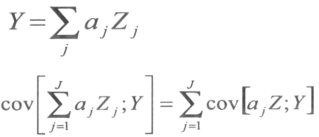
The left-hand side is the covariance between Y and itself, and represents the variance of Y. Then:

Dividing by: σ²(Y)

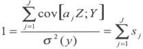
Where, each s_j; is given by:

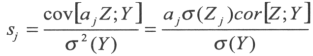
Sj's represents the weighted factorial inequality (FIW) and the lump-sum of all of these explanatory factors equals 1. Every s_j can be decomposed as follows: The years of education greater explains the income inequality:

•     As higher is the regression coefficient to Education

•     As higher is the standard deviation of the years of education

•     As higher is the correlation between education and income (covariance)

Fields explain that this decomposition applies to other commonly used inequality measures; such as the Gini Coefficient, the Atkinson Index, the generalized entropy family indexes, also the log-variance ones.

 

A.2 Building the Social Mobility Index

The Fields Decomposition allows us to judge the importance of each explanatory variable through the weighted factorial inequality (FIW). For example, if the FIW accounts for 0.07 means that 7 per cent of the total variation is explained by this particular variable. Therefore, if we account for the maximum years of education of the parents (Emax) and the per capita household income (Ipc), controlled by adult equivalences; these variables account for the family initial conditions. If the family initial conditions are important, then the social mobility index is low; the opposite applies. Thus, Andersen (1993) defines de SMI as:

SMI = I - (E_max + I_pc)

1 Appendix A follows the appendix provided in Andersen (2003)