TRABAJO DE INVESTIGACIÓN

 

Exchange Rate Volatility in Emerging Markets
The Chilean Case*

 

 

Juan R. Castro**

 

 

---

Abstract

This paper empirically investigates the volatility of the Chilean pegged exchange rate regime using a target zone model. Using the ARCH model, this paper tests the exchange rate volatility in the presence of different levels of foreign reserves and other macro shocks. it is found that the domestic credit, domestic debt, and foreign debt have the largest volatility of the variables tested when compared with other fundamental variables. The variance of the exchange rate is heteroskedastic but not persistent, which implies that the exchange rate was stable, probably moving within the band. The exchange rate volatility fluctuates more with domestic and foreign debt than with the other variables tested.

---

Resumen

El documento realiza una investigación empírica sobre la volatilidad del régimen cambiario chileno (pegged exchange rate regime), utilizando un modelo de Zonas Objetivo. Mediante el uso del modelo ARCH, el documento realiza pruebas sobre la volatilidad del tipo de cambio en presencia de diferentes niveles de reservas internacionales y otros shocks macroeconómicos. Los resultados muestran que el crédito doméstico, la deuda interna y la deuda externa tienen el mayor impacto sobre la volatilidad de las variables estudiadas, especialmente cuando se comparan con otras variables fundamentales. La varianza del tipo de cambio es heterosedastica pero no es persistente, lo que implica que la tasa de cambio es estable, probablemente cuando oscila entre dos bandas. La volatilidad del tipo de cambio fluctua en mayor medida ante cambios en la deuda interna y externa, que con las otras variables utilizadas.

---

 

 

1. Introduction

The exchange rate has been used by many countries as a tool to control inflation, promote economic growth, increase the balance of payments, and attract foreign investment. There are three different types of exchange rate regimes: floating, pegged (fixed, but adjustable), and fixed. In this paper, we will deal with the last two types of exchange rates, pegged moving within a band, and fixed. Industrialized countries mainly use floating exchange rates. A number of developing countries use the pegged exchange rate, and only a few countries use the fixed exchange rate regime.

In a pegged exchange rate system, the central bank sets target bands where the exchange rate can fluctuate. The central bank, through monetary interventions, makes sure the exchange rate does not exceed pre-established limits. Pegged exchange rates are favored by most developing countries. In the last decade, we have seen a large number of countries using the pegged system for their exchange rate regime. It has been used as the means to manage the instability of their currencies and their level of inflation generated by the uncertainties and constant devaluation. European countries were one of the first to introduce the pegged exchange rate system, followed by several Asian countries such as Indonesia and Thailand. Since the beginning of the 1980s, most Latin American countries have introduced the pegged system as a means to control exchange rate fluctuations.

This paper examines volatility of the exchange rate on an emerging market like Chile. The target zone models used previously for European countries are applied to Chile and test if the target zone implications are observed. It analyzes the performance of the pegged exchange rate in emerging market countries.

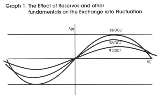
The model studies the effects that foreign reserves and the rate of foreign reserve changes can have in the exchange rate. Different levels of foreign reserve demand are tested to examine if increasing the level of reserves reduces the level of exchange rate fluctuation (see Graph 1).

Where:

R1/DC1 > R2/DC2 > M3/R3, and R1 > R2 > R3, and DC1 = DC2 = DC3
s(t) = f(t) + αEds(t)/d(t)
f(t) = several fundamental variables such as the foreign reserve, domestic and foreign interest rate, terms of trade, and so forth.
R = Foreign reserves, s(t) = exchange rate, f(t) = fundamental,
DC = domestic credit

 

2. The Target Zone of Exchange Rate

The standard exchange rate target zone work began with Krugman (1991) and has become the starting point for almost all the research that followed. Despite the fact that in the early 1980s the European countries introduced their pegged exchange rate system, which allowed the exchange rates to move inside of bands (called target zone), there was no model that could represent the dynamics of the pegged exchange rate before Krugman. Although many emerging market countries have been using pegged exchange rates, which are similar to the target zone system, there is no research on studying the exchange rate target zone in those countries.

The target zone model started from the presumption that the exchange rate, like any other asset price, depends on both current fundamentals and expectations of future values of the exchange rate. According to Krugman (1991), in a target zone regime, the exchange rate at any point in time is determined by,

where s is the log of the price of foreign exchange, given by how many domestic currency units are needed to buy one foreign currency unit, m is the log of the money supply, V is an exogenous shock term incorporating several macroeconomic variables such as shifts in income, velocity, terms of trade, domestic debt, etc. a is a positive coefficient interpreted as interest semi-elasticity of money demand, and the last term, Eds/dt, captures the effect of expected change in the exchange rate. Usually referred to as velocity in target zone literature, the exogenous shock term, v(t), is assumed to follow a random walk with drift:

where u and Φ are constants and dz is the increment of a standard Wiener process.

As an example, for a given level of the current fundamentals, a higher future expected exchange rate (a lower expected future value of the domestic currency) implies a higher exchange rate (a lower value of the domestic currency) today. Conventionally, the exchange rate is defined as the domestic price of the foreign currency, which is the number of domestic currency units per foreign currency unit. Therefore, the exchange rate and value of the domestic currency are inversely related.

The standard target zone model has two crucial assumptions. First, the exchange rate target zone is perfectly credible, i.e., market agents believe that the central bank will maintain the exchange rate within the specified band. Second, the target zone will be defended with marginal interventions only. That is, the money supply is held constant and no interventions occur at all as long as the exchange rate is in the interior of the exchange rate band. When the exchange rate reaches the weak edge of the band, the money supply is reduced to prevent the currency from weakening further, and vice versa when the exchange rate reaches the strong edge of the band.

 

3. Chile's Target Zone

This paper empirically investigates the credibility of the Chilean pegged exchange rate regime using the target zone model implications. The target zone theory has only been tested using data from European countries. However, several countries from Latin America and Asia have also used target bands similar to the bands established previously by the European Monetary System.

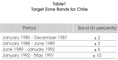
Chile is a good case because has been using the pegged exchange rate since 1979. In 1985, the Chilean government introduced a nominal exchange rate system characterized by a crawling band similar to the previous European target bands. Table 1 shows the different periods and band width during fourteen years.

*This table presents the upper and lower bands of the exchange rate target zones for Chile between 1985-1997. The band width was tabulated from information provided by Bosworth, Dornbush, and Laban. In their book "The Chilean Economy." From 1979 to 1983 the exchange rate was fixed. In 1985, with the purpose to maintain the international competitiveness of exports, Chile adopted a crawling band (target zone) system, allowing the exchange rate to move within the bands. By late 1989, the central bank decided to increase the width of the band to ± 5 percent after inflation had climbed to 30 percent, imports had grown at 35 percent, and the GDP had grown at 10 percent. By the end of January 1992, a rapid accumulation in foreign reserves put pressure on the exchange rate, moving it to the floor of the band. The central bank decided to counterattack the domestic exchange rate appreciation by increasing the band from ± 5 to ±10.

During the second period, the band width increased at the end of June 1989 from ± 3 to ± 5. This was the result of economic overheating. During this second period, the inflation climbed to 30 percent, imports grew at 35 percent, and the GDP grew at 10 percent. The central bank decided to expand the band by two percent points and increased the interest rate close to 3 percentage points, from 6.9 percent to 9.7 percent. By the end of January 1992, a rapid accumulation in international reserves put increasing pressure on the exchange rate, moving it to the floor of the band. The central bank decided to counterattack the domestic exchange rate appreciation by increasing the band from ± 5 to ± 10 percent.

 

4. Methodology

In this paper, we test exchange rate volatility. In a target zone scenario, testing volatility is crucial. According to basic target zone literature, the volatility of the exchange rate diminishes when it gets closer to the bands. The second generation of target zone models asserts that the volatility of the exchange rate increases when it approaches the upper band, since speculators believe the monetary authority intervention is not credible. The zero target zone implies that the volatility diminishes and the intervention is credible. Following Engle (1982), we use the ARCH (Autoregressive Conditional Heteroskedasticity) procedure to test an exchange rate model and to identify the determinants of exchange rate volatility.

 

5. Data

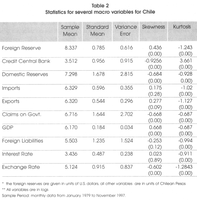
This chapter uses monthly data from Chile for January 1979 to November 1997. The data used consists of foreign reserves, credit from the central bank, domestic reserves, imports, exports, claims on the government, GDP, foreign liabilities, domestic interest rate, and foreign interest rate. Using the above variables, several composite variables are created, such as the reserve ratio, terms of trade, domestic debt, and international debt. The reserve ratio is given by the foreign reserve and domestic credit ratio. Terms of trade is the ratio of exports and imports, and the domestic debt and international debt are given by the claims on government divided by GDP and international liabilities divided by GDP, respectively. The lending rate was used for domestic interest rate and the U.S. Treasury Bill for the foreign interest rate. These data were taken mainly from the IFS CD-ROM. The GDP was taken from the Chilean central bank published through the Internet. The data used is converted to natural logs. Table 2 presents the statistics of these variables.

 

6. Using ARCH to Examine the Exchange Rate Volatility

The analysis of volatility is essential in the study of target zones and other monetary systems. The basic target zone assumes that the volatility diminishes when the exchange rate approaches the bands. The second generation of target zones assumes that the exchange rate volatility is time variant, causing the target band to expand or the exchange rate to realign to a new central parity. The zero target zone or currency board assumes that the volatility is low or nearly constant. Most of the papers in the target zone literature have concentrated on the testing for realignments and the devaluation risk, most notably Delgado and Dumas (1993), Svensson (1991), and Werner (1995). In this section, we concentrate on testing the volatility of the exchange rate and the main components that influence its volatility. We want to determine if the exchange rate has a constant or homoskedastic conditional variance, or if the variance is time variant or heteroskedastic. If the variance is constant, it means there is a linear relationship between the exchange rate and other fundamental variables. Heteroskedastic variance will imply a non-linear relationship between the exchange rate and other fundamental variables.

To test for volatility, we use the ARCH model. Engle (1982) developed the ARCH model as a tool to test for volatility. The model consists of two steps. The first step is to find if there is an ARCH effect, if the data follows an ARCH process. If such effect exists, then the parameter estimations are found and used to obtain the volatility of the variables. We also examine what variables have a stronger effect inferring the existence of time variant variance.

The standard ARCH regression model can be written as:

where X_t are the observable variables, and Y_t-1 is used to test for stationarity. The marginal distribution will reveal if the y_t (exchange rate in our case) volatility is reduced when it approaches same specified target. If ε_t exhibits fatter tails than normal, it indicates that there is concentration of the marginal distribution of the exchange rate near the bands and reduced volatility, and consequently a non-linear distribution between the exchange rate and the observable variables, X_t. The fatter tails can also indicate that the distribution of the exchange rate is U-shaped.

Engle (1982) proposes a test for the existence of the ARCH effect. If there is no ARCH effect, the regression will have little explanatory power, so the coefficient of determination (i.e., the usual R² statistics) will be quite low. With a sample of T residuals, under the null hypothesis of no ARCH effect, the test statistic TR² from maximum likelihood estimation converges to chi-square distribution. If TR² is sufficiently large, then we can reject the null hypothesis of no ARCH effect. On the other hand, if TR² is sufficiently low, then we can conclude no ARCH effect. The lack of ARCH effect denotes that the variance is not time variant and that the variance may be homoskedascic. Having a constant variance helps us to predict that the error term of the variables may be white noise and the relationship of the variables is linear. Following standard ARCH regression presented on (3), the ARCH regression for the exchange rate can be written as:

where the exchange rate, S_t, depends on the past values of the exchange rate, S_t-1, reserve ratio, R_t/DC_t, the ratio between exports and imports or terms of trade, To T_t, domestic debt, DD_t, international debt, ID_t, and the error term ε_t. S_t is stationary when S_t-1 is less than one. Allowing the variance to depend upon the information available by the exogenous variables, and assuming conditional normality, we can specify the evolution of S_t as:

where X_t = R_t/DC_t, ToT_t, DD_t, and ID_t , and g_t is E(S_t/S_t-1, X_t), ε_t ~ N(0, h_t), and h_t = α₀ + 2∑α₁(ε_t-1)², where i = 1 ...4, i.e. for each exogenous variable.

Although ε_t is white noise, successive values are not independent because they are related with past values through higher moments. If we want to forecast one step ahead for the conditional mean and conditional variance, then we have:

In order to have a positive variance, we need to restrict α₀ and α_i to be positive; and to have a stable variance, we need 0 < α_i < 1. The parameter α_i is important because it shows if the volatility is persistent If the value of α_i is closer to 1, it will imply that the volatility is persistent, that the exchange rate might not have been mean reverting and it might move outside from the pre-established bands. In such case, realignment or devaluation will be necessary, or the bandwidth may be increased to cover the new exchange rate. On the other hand, if α_i is small (i.e. closer to zero), it will suggest that even though the conditional variance is heteroskedastic, it is not persistent and the exchange rate may move back to its mean. A small α_i will also suggest that the small volatility may be the response caused by a small shock or intervention. If α_i is equal to zero, the estimated variance, h_t, is the constant α₀,. Otherwise, the conditional variance of S_t evolves according to α_i. If α_i(ε_{t +} 1)² is large, the variance of ε_t will be large. So, if the variance is conditional heteroskedastic, this implies that the exchange rate follows an ARCH process. In that case, we can capture periods of tranquility and volatility in the exchange rate.

 

7. Empirical Evidence

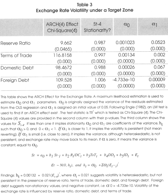
We ran a maximum likelihood estimation to estimate the coefficients of the exchange rate, and the parameters α₀ and cij, to obtain the ARCH variance. The value assigned to α₀ is obtained from the variance of the residuals estimated from the OLS regression, and to α_i was assigned 0.05 (a small number). The Lagrange multiplier test for ARCH(1), ARCH(2), and ARCH(3) were not significant, but the test for ARCH(4) yielded significant values. The following estimations are obtained:

where the values in parentheses are the p-values. The coefficient for the lagged exchange rate is positive and less than one, which implies stationarity. The positive point estimates support the ARCH assumptions, and the value of α_i = 0.0211 suggests that volatility is not persistent, but rather it is a small heteroskedastic variance. This finding tells us that the exchange rate volatility was small for Chile's data.

Table 3 shows that the ARCH effects are given by the reserve ratio, domestic debt, and international debt.

For example, we can observe that the ARCH (4) effect test for the reserve ratio is of 9.6620 with a p-value of 0.04465, α₀ is 0.001023, a, is 0.0523, and S_t-4 is 0.987, implying stationarity. We can observe that the variances of these variables are very low, suggesting a low impact on the exchange rate volatility. When the exchange rate with a lag of four was ran against the foreign debt, the value of the coefficient is greater than one, i.e., S_t-4 = 1.006, suggesting non-stationarity. Also, the value of the constant is negative, i.e., α₁ = -4.733e-10, which violates the positive restriction for the ARCH coefficient. These results indicate that the volatility of the exchange rate is influenced by the reserve ratio, domestic debt, and terms of trade. A reduction of domestic debt and an increase of the foreign reserve will reduce the exchange rate volatility.

 

8. Conclusion

We examine the effects of foreign reserves and other fundamental variables on the exchange rate volatility. We found that the domestic credit, domestic debt, and foreign debt have the largest volatility of the variables tested when compared with other fundamental variables. The volatility of the exchange rate was tested using the ARCH model. We found that the variance of the exchange rate is heteroskedastic, but not persistent, which implies that the exchange rate was stable, probably moving within the band. The exchange rate volatility fluctuates more with domestic and foreign debt than with the other variables tested.

 

Notes

* We would like to thank Frank Lopez, Naka Asuyuki, Oscar Varela, and Gerald Whitney, from University of New Orleans, for helpful comments and suggestions.

** School of Business. Le Tourneau University.

 

References

Bosworth Barry, Rudiger Donbusch and Raul Laban. 1994. The Chilean Economy, Policy. Lessons and Challenges. The Brookings Institution, Washington, D.C.

Delgado, Francisco and Bernard Dumas. 1993. "Monetary contracting between central banks and the design of sustainable exchange rates zones". Journal of International Economics, 34, 201-224.

Engle, Robert F. 1982. "Autoregressive Conditional Heteroscedasticity with Estimates of the Variance of United Kingdom Inflation". Econometrica, 50:987-1007.

Flood, Robert, and Andrew Rose. 1991. "An empirical exploration of Exchange rate target zones". Carnagie-Rochester Series on Public Policy, Fall, 35, 7-66

Krugman, Paul R. August. 1991. "Target zones and Exchange rate dynamics". Quarterly Journal of Economics. Vol. 106, N° 3, 669 - 682.

Krugman, Paul and Marcus Miller. 1991. "Speculative Attacks on Target Zones". Oxford: Oxford University Press.

Lewis, Karen. 1995. "Occasional Interventions to Target Rates". The American Economic Review. September P. 691-715.

Svensson, Lars E. 1991. "Target zones and interest rate variability." Journal of International Economics. N° 31, 27 - 54.

Svensson, Lars E., 1994. "How long do Unilateral target zones last?". Journal of International Economics. Vol. 36, 467 - 481.

Werner, Alejandro M. 1995. "Exchange rate target zones, realignments and interest rate differentials Theory and evidence". Journal of International Economics. Vol. 39, 353 - 367.