TRABAJO DE INVESTIGACIÓN

 

Bolivia: Impact of Shocks and Poverty Policy on Household Welfare*

 

 

Gover Barja Daza, Javier Monterrey Arce, Sergio Villarroel Böhrt**

 

 

---

Summary

This paper evaluates the short term impacts on poverty of pro-poor expenditure and total social expenditure during the 1998-2002 period of Bolivian economic recession. Observed characteristics of recession are simulated by the combined effects of negative terms of trade shock, reduction in foreign saving flows and low output growth. Evaluation is performed by simulating the impacts of shocks and social expenditures in an environment of low growth: i) on macro aggregates of consumption, income, saving and prices (based on a simple static 1-2-3 model), ii) on household income and consumption levels, and iii) on consumption based poverty indicators. The following were main results from experiments:

The terms of trade shock had greater negative impact on household income then reduction in foreign saving flows. In contrast, reduction in foreign saving flows had greater negative impact on household consumption then the terms of trade shock. The head count ratio has been greater from reduction in foreign saving flows then from the terms of trade shock. Poverty gap and poverty ¡ntensity has concentrated in rural areas, being greater from reduction in foreign saving flows then from the terms of trade shock.

The combined positive effects from observed social expenditure policy and effort in an environment of low output growth, did not compensate the combined negative impacts from the experienced terms of trade shock and reduction in foreign saving flows.

These conclusions show that under macroeconomic disequilibrium poverty reduction efforts become policies of poverty containment or safety net programs. Poverty reduction is a long term objective that requires long term commitment for an environment on macroeconomic stability.

---

Resumen

Esta investigación realiza un análisis de los impactos de corto plazo en la pobreza de los gastos pro-pobres y el gasto social total en el período de la recesión económica boliviana (1998-2002). Las características observadas de la recesión fueron simuladas a través del efecto combinado de shocks negativos de términos de intercambio, reducción de los flujos de ahorro externo y bajo crecimiento económico. El análisis se desarrolló a través de la simulación de los impactos de los shocks y el gasto social en un entorno de bajo crecimiento: i) en los agregados macroeconómicos del consumo, ingreso, ahorro y precios (basado en un modelo estático simple 1-2-3); ii) en los niveles de ingreso y consumo de los hogares y iii) en indicadores de pobreza basados en el consumo. Los siguientes son los principales resultados de las simulaciones:

El shock de términos de intercambio tiene un impacto negativo mayor sobre el ingreso de los hogares que la reducción de los flujos de ahorro externo. En contraste, la reducción de los flujos de ahorro externo tiene un impacto negativo mayor en el consumo de los hogares que el shock de términos de intercambio. El indicador de pobreza 'Head Count Ratio' ha mostrado mayores incrementos ante la reducción de los flujos de ahorro externo que por shocks de términos de intercambio. Tanto la brecha como la intensidad de la pobreza se han concentrado en áreas rurales, causadas mayormente por la reducción de los flujos de ahorro externo que por shocks de términos de intercambio.

Los efectos positivos fruto de la combinación de las políticas de gasto sociales observadas con el esfuerzo realizado en un entorno de bajo crecimiento del producto no compensan los efectos negativos conjuntos de los impactos de los shocks en términos de intercambio y reducción de los flujos de ahorro externo.

Estas conclusiones muestran que, ante desequilibrios macroeconómicos, los esfuerzos para reducir la pobreza se convierten en políticas de contención de la pobreza o bien programas de redes de seguridad. La reducción de la pobreza es un objetivo de largo plazo y requiere un compromiso también de largo plazo para mantener un entorno de estabilidad macroeconómica.

---

 

 

1. Introduction

This paper develops a simple static model that connects a small open economy framework to the Bolivian poverty reduction strategy. The main objective is to evaluate the short term impacts on poverty of pro-poor expenditure and total social expenditure more generally, during the 1999-2002 period of economic recession. Secondary objectives are to establish: 1) the degree and channels through which external shocks impact poverty reduction efforts, 2) the degree and channels through which stabilization policy complement and/or conflict with poverty reduction efforts, and 3) identify main lines of recommendations for public policy. An implicit objective is to evaluate performance of the market led model, built since 1985, in poverty reduction under shocks and recession.

What are the connections between the macro economy, shocks and poverty reduction? As a consequence of shocks to the economy, the decrease in growth and aggregate consumption, saving and investment, expressed in changes in overall prices, wages and profits, will have an impact on welfare expressed in changes in household income, consumption and overall poverty and its structure.

A starting idea was that poverty reduction is a long term objective that requires a long term commitment for an environment on macroeconomic stability. Poverty reduction efforts and policy will have its full impact in poverty reduction instead of poverty containment only if the macro environment is stable. Moreover, a higher degree of economic instability could genérate economic forces that reduce overall welfare with greater impact on poor.

A model of the 1-2-3 type is developed for the macroeconomic aspects and the introduction of shocks and pro-poor expenditure policy. Household income, consumption and poverty indicators to evaluate the impact of shocks and expenditure policy are based on 1999 household data. The reason for divergence in base years between the macro model and household data is that the MECOVI survey, designed to study poverty, began in 1999.

Besides this introductory section, the second section describes some key features of recent Bolivian macroeconomic performance in order to identify main shocks experienced during the period of economic recession. Also establish their magnitude as well as the magnitude of poverty reduction effort in terms of expenditure. The third section presents the macro model (static, simple and flexible of the 1-2-3 type) with structure and parameters that best represent the Bolivian economy in 1998. This year is selected as the base year because it is the one just before the beginning of economic recession and because it is the last year of high growth performance accomplished by the market led model that resulted from structural reforms since 1985. Based on 1999 household survey data, the fourth section presents household income and expenditure structure, as well as poverty indicators accomplished by the market led model.

The fifth section connects the macro model to household data through aggregate income and consumption. This connection is used to evaluate the impacts of shocks and poverty reduction policy on household welfare and poverty. First, macroeconomic impacts from shocks and poverty reduction policy are simulated in order to generate changes in aggregate income and consumption. Second, these changes are used together with household data to simulate the effect of shocks and policy on household income and consumption levels by quintiles and areas, and also their effect in terms of changes in poverty indicators by areas. Conclusions, limitations and policy implications are presented in the last section.

 

2. Recent performance of the Bolivian economy

Bolivian efforts for economic development can be summarized in the first structural reform of 1985-89 aimed at stabilization and market liberalization policies, and the second structural reform of 1994-97 based on privatization and regulation policies. Among the most important implications of structural reforms is the construction of a market led growth model where the government's roll is primarily concentrated in social expenditure and regulation. Bolivian efforts in poverty reduction in particular can be summarized in the Bolivian strategy for poverty reduction (PRSP, 2001) originally based on the distribution of HIPC resources, but later amplified to the concept of pro-poor expenditure which began much earlier during the 90's (UDAPE, 2003).

The following figures provide a brief review of performance of the Bolivian economy. Figure 1 shows that structural reforms had a positive impact on economic growth allowing growth rates up to just above 5 per cent until 1998. During this period a common expression was that Bolivia needed much higher growth rates in order to have some significant effects on poverty reduction. Then at the beginning of 1999 the economy experienced a sudden stop and entered a period of recession and slow recovery until today. Finally a growth rate just above 3 per cent during the first semester of 2004 may be the awaited indication that recovery is to stay and speed up.

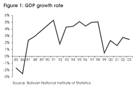
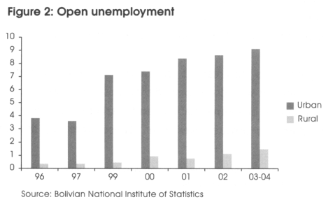
Figure 2 shows that the growth period also had a positive impact in the open unemployment rate which by 1997 was at it lowest of 3.65 per cent in urban areas and 0.25 per cent in rural areas. From 1999 on, the open unemployment rate has grown continuously even showing a disconnection with initial economic recovery. The reason for this is that economic recovery is largely explained by new oil and natural gas exports, a sector that is not employment intensive. Although government had additional income from oil and gas rents, these have not prevented a fiscal deficit of 9 per cent of GDP by 2002 and could not prevent a contractionary fiscal policy due to a significant net drop in government income, caused by recession, against rigid government expenditures.

As a consequence the impact of growth on poverty is expected to have reversed after 1999. At the same time, greater pro-poor expenditure under the Bolivian Poverty Reduction Strategy (BPRS) and greater social expenditure more generally is expected to have helped with poverty containment. However, one can not help to wonder how the Bolivian economy could have evolved if macroeconomic stability was maintained, together with a 5 per cent growth and current poverty reduction resources. One can not help to ask what happened in early 1999 that changed the Bolivian growth path and history. One answer is the accumulation of several events in a moment in time when the key second structural reforms where only beginning to take hold. What were those events?

Foreign direct investment (FDI) in Bolivia has followed a pattern similar to that observed throughout Latin America and the Caribbean (Eclac, 2004). After reaching its highest level and sudden stop in 1999 (see Figure 3), the following years FDI drops back to its early levels, having a large impact on total investment, particularly by 2003. However, total investment (public and private) reached its highest in 1998 and its drop in 1999 is explained by the sudden stop of private domestic investment¹.

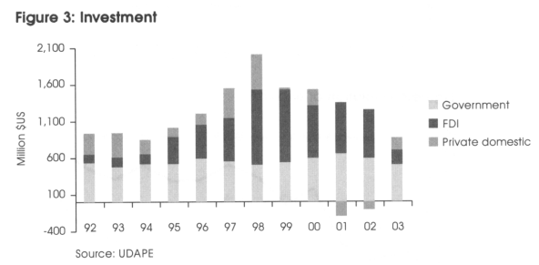
FDI was expected to diminish as capitalized firms fulfilled their investments commitments, however it was also expected that these firms would continue investing given an environment of economic stability and market led growth, as well as induce the increase in domestic private investment. These were key assumptions for the consolidation of a private led market oriented economy in Bolivia. When the time came, the economic environment had deteriorated due to external and internal factors.

Contraction in economic activity and aggregate demand can also be observed from the behavior of the banking system (see Figure 4). By 1998 the system reached its highest level of activity, in 1999 it experienced a sudden stop and even decreased, then the following years show a substantial drop in assets (largely loans) and liabilities (largely deposits) toward their early levels. The drop in liabilities is explained by important deposit withdrawals due to an environment of higher risk and uncertainty that resulted from economic contraction accompanied by a deteriorated social environment, this last being a main source of internal shock. Part of those withdrawals may have left the economy as capital flight, an event that has also been observed throughout Latin America during this period.

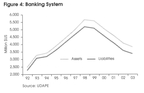
Figure 5 shows the large drop experienced in the bilateral exchange rate with Brazil in 1999 and later in the bilateral exchange rate with Argentina in 2002. However, the multilateral real effective exchange rate (REER) shows that real depreciations in the bilateral exchange rate with other countries, particularly the United States with whom Bolivia has its largest trade, has somewhat helped in compensating those drops.

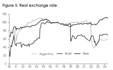
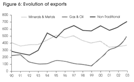
Figure 6 presents the evolution of the value of exports in million $US in its three global categories. It shows a decreasing tendency in exports of primary minerals and metals, with a drop also in 1999 but its lowest level in 2001. This is explained by the long term decreasing tendency of international prices of Bolivian mineral exports. It also shows 1999 as the year of lowest exports of oil and natural gas. Natural gas exports to Argentina ended in early 1999 and later in the same year began natural gas exports to Brazil. Although non-traditional exports presents a general tendency to increase and contribute to diversification of Bolivian exports, in 1999 those exports also experienced a slow down compared to previous two or three years.

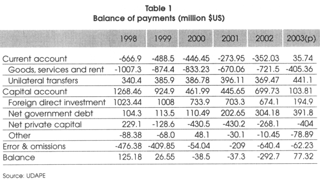
How did the above affect the balance of payments? Table 1 shows that although the capital account (foreign saving flows) compensated for traditional current account deficit, its flow levels had decreased substantially after 1998. Between 1998-2002, the capital account decreased by 55 per cent explained by the combined effect from 66 per cent decrease in FDI, 117 per cent decrease in net private capital and almost three fold increase in new net government debt.

By 1998 the market led growth model helped the government concentrate half of its spending in social expenditure in general (Figure 7) and pro-poor expenditure in particular (15.63 per cent and 10.2 per cent of GDP by 1998 respectively).

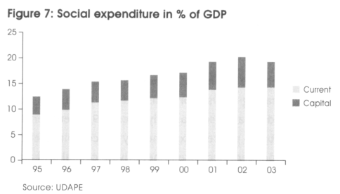
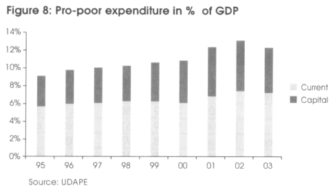
Figure 8 shows that pro-poor expenditure has been increasing during economic recession, reaching its highest level so far by 2002 (13.1 per cent of GDP), with the characteristic that current expenditure has been greater then capital expenditure.

As Figure 9 shows, this was accomplished in a period were government income (Yg) decreased due to recession, generating a fiscal deficit of 9 per cent of GDP by 2002 (DF) and forcing contraction of government's current spending (GCg) in general but not of government investment (Ig).

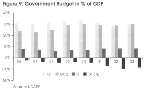
Pro-poor expenditure includes total current and capital expenses on education, health, rural development, housing and sanitation. Social expenditure includes, in addition to pro-poor expenditure, pension payments and contributions, university transfers and "benemeritos". Its financing comes from government income, mostly for current expenses, and from foreign credit and donations, HIPC resources and the National Compensation Program, mostly for capital expenses.

A question is whether pro-poor expenditure or more generally social expenditure has been able to compensate welfare losses caused by shocks to the economy. Who in society were affected the most and by what magnitude. What would have been the magnitude of welfare gains if the economy did not experience external and internal shocks. These are among the question this paper tries to answer strictly during the period of economic recession. The market led model that is put to a test during this period must be evaluated with a longer vision, which is not done here. However, here we can mention some of the latest papers that evaluate its performance.

Based on a general equilibrium model, Thiele and Wiebelt (2003) conclude that Bolivian economic growth for the period 1985-99 cannot be called pro-poor, because it bypassed traditional agriculture and the urban informal sector where most of the poor earn their living. They also conclude that the goals of the Bolivian poverty reduction strategy can be reached only under optimistic assumptions, its performance fall short of expectations once external shocks are taken into account (such as El Niño). The evolution of poverty is likely to remain uneven, with considerable improvements in urban areas and a high degree of persistence in rural areas. The differentiated impact of the growth process on household income, observed for Bolivia, is likely to be the rule rather then the exception.

Barja and Urquiola (2003) and Barja, McKenzie and Urquiola (2004) conclude that privatization in infrastructure sectors (telecommunications, electricity and water services) has improved net consumer welfare in main urban areas (with larger impact on the lower income quintiles). Based on regression analysis they show that welfare gains occurred because greater access to services has outweighed welfare loses from some price increases. Based on administrative data they conclude that infrastructure sectors (including the oil and gas industry) had gain in internal efficiency and investment and by large the oil and gas industry attracted most of foreign investment and also generated the greatest prospect for future growth. However, privatization was oversold in the employment and household income front, particularly beyond main urban areas, and has been rejected by the majority of population by the perception that its benefits had reached the few.

Based on administrative data, Garron, Capra and Machicado (2003) show that while privatization did not have significant impact on profitability, it increased operating efficiency, reduced employment at the firm level and decreased fixed assets. Based on regression analysis they show that privatization itself has been a significant factor in explaining the improvement of operating efficiency. Other significant factors are the size of firms, the presence of regulation and quality of management.

Based on a recursive-dynamic general equilibrium model, Jemio y Wiebelt (2003) conclude that Bolivia is highly vulnerable to external shocks in the form of decreasing world prices of exports and decreasing foreign direct investment and portfolio flows. Moreover, the spontaneous adjustment is severely restricted due to limited possibilities of substitution in the markets of goods and factors, as well as institutional restrictions about portfolio alternatives. Structural characteristics of the economy also affect the outcome of anti-shock policies. An expansionary fiscal policy is not feasible due to its negative impact to the balance of payments and fiscal equilibrium. In contrast, a nominal depreciation of the Boliviano does increase growth and employment, and also improves the fiscal and external balance. Despite structural rigidities, a nominal depreciation does generate a real depreciation sufficiently strong to stimulate the necessary resource reallocation for an effective adjustment. Regarding the poverty reduction efforts, they conclude that the combination of foreign debt relief (HIPC II initiative) with a fiscal expansion does generate greater rates of growth, lesser fiscal and external disequilibrium and lesser unemployment.

Based on regression analysis with household survey data, Andersen (2003) uses the determinants of education gap to show very low social mobility in Bolivia. Low social mobility helps explain poverty persistence over time and may be due to inadequate public education, corruption, marriage selectivity, insufficient rural-urban migration and labor market imperfections.

The Bolivian Poverty Reduction Strategy Paper (PRSP, 2001) represents the initial government policy in this front and has as main premise that poverty, inequity and social exclusion are the most severe problems that affect democracy and governance in Bolivia. The strategy was originally funded on HIPC II resources, distributed to Bolivian 314 municipalities based on criteria defined on the National Dialogue (2000), and who in turn invest in social projects. Based on administrative data, the latest government evaluation of the strategy (UDAPE, 2003) reveals several internal and external sources of funding besides HIPC II and introduces a pro-poor expenditure measurement which was traced back to 1995. Evaluation of the strategy already suggests change in its vision, from a strictly social assistance to the poor view to an employment and income generation view through investment in small producer projects.

 

3. A simple macro model

3.1. Analytical framework

The analytical framework of the 1-2-3 model (extended version with government and investment²) is presented in Devarajan, Lewis and Robinson (1990), Devarajan, Lewis and Robinson (1993), Devarajan et al. (1997) and Devarajan and Go (2002). A brief description is presented here and in Appendix 1.

This model refers to a single country with a small open economy that produces two goods: a non-traded domestic good D and an export good E. From the consumption point of view, the country consumes an import good M, which is not produced in the economy, and the domestic one. Some of its basic characteristics and assumptions are the following:

- The model has four actors: a producer, a household, the government and the rest of the world.

- It is a static model for a given growth rate of the economy with no intertemporal elements.

- The model identifies an equilibrium relationship between the real exchange rate and the balance of trade, which is fixed exogenously.

- The model contains no monetary elements and any solution to the system depends only on relative prices (it is a "real" model).

- The model takes the two factors of production (capital and labor) as constant, and it doesn't consider any imported or domestic intermediate goods.

- The domestic and export goods are imperfect substitutes.

- The output of the domestic good is an imperfect substitute for imports in consumption.

- World prices of exports and imports are fixed exogenously (small country assumption equivalent to price takers).

- Aggregate production is fixed, which is equivalent to assuming full employment of all primary factor inputs.

The model can be summarized in the following simple programming model (without government), where a consumer utility function or absorption is maximized, which is equivalent to maximize social welfare, subject to: i) a technology constraint that represents the maximum combination of output, given a fixed proportion of production factors (production possibility frontier); ii) a balance of trade constraint that is determined exogenously; and iii) a market clearing condition for the domestic good "D".

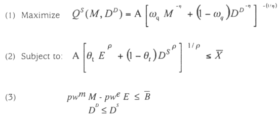
3.2. Elasticity estimation to Bolivia

Table I.1 in Appendix 1 presents the first order conditions of consumer utility maximization (equation 4) and producer profit maximization (equation 3). Both equations represent long term relationships among the variables of interest, which include the elasticity of substitution and the elasticity of transformation. Both elasticities were estimated for the Bolivian case based on quarterly data for the period 1990-2002. Appendix 2 presents the methodology, strategy and econometric procedure followed for elasticity estimation. The estimated cointegrating equations are the following;

The CES model result suggests on average an elasticity of substitution of 0.45 in the consumption of the import good relative to the domestic good when there is a change in their relative prices. The negative sign of the slope indicates that, when the price of the import good increases while the price of the domestic good remains constant, consumption of the import good will decrease and consumption of the domestic good will increase.

The CET model result suggests on average an elasticity of substitution of 0.60 in the production of the export good relative to the domestic good when there is a change in their relative prices. The positive sign of the slope indicates that, when the price of the export good increases while the price of the domestic good remains constant, production of the export good will increase and production of the domestic good will decrease.

 

4. Evaluating household welfare and poverty

4.1. Computation of aggregate consumption

Table 2 summarizes computation of aggregate consumption and its structure³. In 1999 Bolivia had 1.85 million households, 62.7 per cent in urban areas and 37.3 per cent in rural areas, reflecting the relative importance of urbanization in the country⁴. Aggregate consumption in urban areas was 2.96 times greater than in rural areas, showing an important difference between geographical areas.

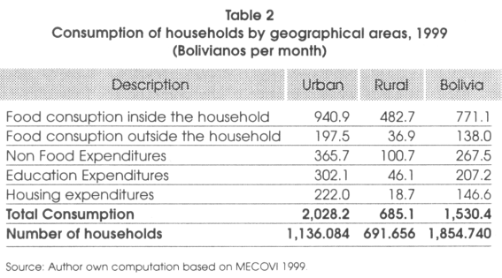
The ratio of food consumption inside the household with respect to the total consumption represents 46 per cent in urban areas and 70 per cent in rural areas.

Education, housing and non food expenditures in urban areas are greater than rural areas, reflecting better access to services and markets in urban areas.

Table 3 further disaggregates the structure of consumption by quintiles and areas. At the national level, the consumption of the richest quintile is 11.6 times greater than the poorest quintile; 9.6 in urban areas and 10.1 in rural areas.

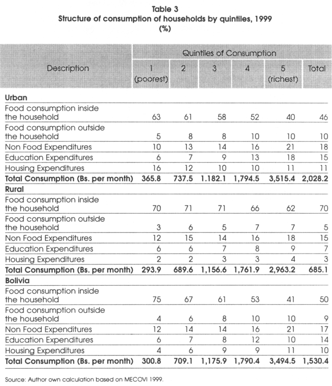
Engel's law (the share of food consumption decreases in richest households) is evidenced inside the urban and rural areas. Comparing the first four quintiles, there are small differences in the structure of consumption, but the last quintile presents bigger expenditures in non food and education expenditures. Differences on extreme quintiles show inequality and polarized characteristic of consumption in Bolivia.

Curiously, the share of housing expenditure in the poorest households is too high in urban areas, this may reflect efforts of the poorest households to access basic services (e.g. water, electric energy).

4.2. Computation of the aggregate income

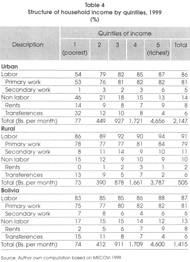
Table 4 is the computed structure of household labor and non labor income by quintiles, where aggregate labor income from primary and secondary sources was computed without extraordinary income. Primary work is the most important source of labor income in urban and rural areas, with increasing importance for the higher income quintiles. Secondary work is a relatively more important source of labor income in rural areas, while non labor income from rents and transferences are relatively more important in urban areas, particularly for the lower income quintiles.

4.3. Poverty indicators

Table 5 presents the computed poverty indicators. The headcount ratio adjusted by Adult Equivalent Scale (AES), at the national level indicates that 41.4 percent of Bolivian households were poor in 1999, that is, they consume under the poverty line. This indicator changes dramatically when comparing urban (23.7 per cent) with rural areas (71.5 per cent).

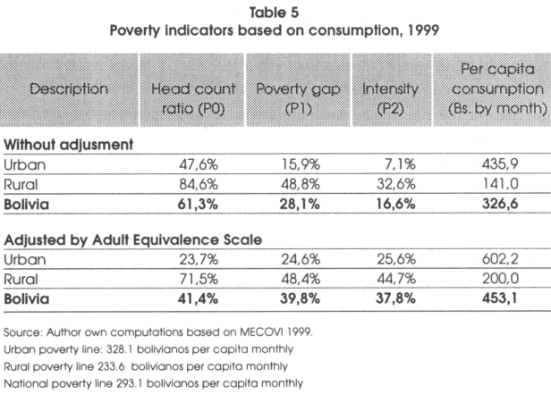
The poverty gap adjusted by AES at the national level indicates that the poor households have a mean shortfall of 39.8 per cent of poverty line value and require on average an additional per capita consumption of 116.5 bolivianos per month to overcome their poverty condition. This indicator also shows large differences when comparing the depth of poverty between urban (24.6 per cent) with rural areas (48.4 per cent).

The intensity or severity of poverty adjusted by AES at the national level indicates an average of 37.8 per cent degree of inequality among poor households .The severity of poverty is greater in rural areas than urban areas, reflecting less inequality between poor people in urban areas and more in rural areas.

It is important to notice that these computations differ from official indicators for three reasons:

i) The official welfare indicator is a mix of income (in urban areas) and consumption (in rural areas). This may not be a better conceptual definition since income and consumption have different implications.

ii) INE's definition of consumption includes health expenditures and estimations of durable goods. In the case of durable goods, the primary source of information is not consistent and has a subjective basis.

iii) The official welfare indicator is not adjusted by Adult Equivalence Scales.

Comparing results of Table 5, the national adjusted Head count ratio is smaller in 19.9 per cent compared to the unadjusted indicator. The AES adjustment has a notably effect especially in poorest and households of big size. The poverty gap is deeper in urban areas then was originally thought with the unadjusted measure, however, the unadjusted measure did well in rural areas. Also inequality among the poor is greater in urban and rural areas then was originally thought with the unadjusted measure.

 

5. Impact of shocks on household welfare

This chapter is developed in two sections; first the 1-2-3 Model is used to simulate shocks to the economy in order to generate information on changes in prices and income. Second, the information on changes in prices and income is then used together with the household data to generate changes in poverty indicators as well as changes in income and expenditures by quintiles.

The objective is to simulate what happened in the 1998-2002 period, with 1998 being the base year and 1999-2002 as the second period which will be compared to the base year (comparative statics). Given that 1998 was the year of highest growth with a correspondent level of welfare accomplished, then the second period would be of loss of welfare, which we want to measure in terms of poverty indicators as well as in changes in income and expenditure.

There are several limitations to this analysis and methodology that must be mentioned:

• Pro-poor government expenditure in education, health and infrastructure for development will have its full returns in terms of poverty reduction only in the long run. Therefore what we measure here is only the short run effects of government expenditures, believing that these expenditures will have a short run effect on overall household income and expenditures.
• Given that the distribution of income and consumption by quintiles is based on a fixed year (1999), which are applied to overall changes in household income and consumption, then this methodology cannot simulate the more complicated process of income and consumption redistribution.
• Given that the 1-2-3 model is built on highly aggregate macroeconomic data, then this model cannot simulate the more complicated process of resource distribution by economic sectors and its consequent effects on household income and expenditures.

5.1 Experiments and macro outcomes

In this section it is of interest to determine the direction and order of magnitude of impact of shocks and pro-poor expenditure policy on the macro economy. The analysis has the following sequence:

• Impact from a terms of trade shock alone;
• Impact from a reduction in foreign saving alone;
• Impact from an increase in total social expenditure alone;
• Impact from an increase in pro-poor expenditure alone;
• Impact from output growth alone;
• Impact from all of the above cases simultaneously, except pro-poor expenditure
• which is part of total social expenditure.

The first external shock considered is a drop in the terms of trade. The Bolivian trade data shows that the economy experienced a 7 per cent drop in its export price index and a 1 per cent drop in the import price index during 1998-2002. The combined effect produces a 6 per cent drop in the terms of trade. The terms of trade are capturing not only the effect of price drops due demand contraction of Bolivian exports but also the price effects of exchange rate crisis in neighboring countries.

The second external shock considered is a decrease in foreign saving. The Bolivian balance of payments data shows that the capital account has decreased in 45 per cent during 1999-2002 compared to 1998. This is explained by three accounts, i) FD1 flows dropped 34.1 per cent during that period, generating a 28 per cent decrease in the capital account balance compared to 1998, ii) net government foreign debt flows have increased by 191 per cent during that period, generating a 15 per cent increase in the capital account compared to 1998, iii) other net private capital has reversed during that period generating a capital flight of 3.1 7 times the positive flow of 1998, generating a 40 per cent decrease in the capital account compared to 1998.

The measurement of pro-poor expenditure came as a result of the need to evaluate the BPRS. These expenditures are part of total social expenditures and part of overall government expenditures. Pro-poor expenditures data show that these have increased in total by 153.06 million $US during 1999-2002 and by 107.36 million $US in its capital component, representing a 17.7 per cent and 31.2 per cent increase compared to 1998 respectively. In the 1-2-3 model this was introduced as an increment of government consumption by 12.7 per cent and an increment of foreign grants by 51.4 per cent respectively. Total social expenditures data show that these have increased in total by 250.5 million $US during 1999-2002 and by 108.7 million $US in its capital component, representing a 18.8 percent and 31.8 per cent increase compared to 1998 respectively. In the 1-2-3 model this was introduced as an increment of government consumption by 20.7 per cent and an increment of foreign grants by 52 per cent respectively.

As seen in Figure 1. GDP has grown an average of 1.74 per cent during 1999-2002, this lower growth rate was introduced in the model as an increase in output by 1.74 per cent. Finally all cases of shocks, expenditure policy and low growth were simulated simultaneously to determine the direction and magnitude of their net effect on macro variables.

Table 6 presents the macroeconomic outcome from all simulations in terms of the model's endogenous variables. The first column is the starting situation in 1998 or base year. The second column is the macro outcome from the terms of trade shock alone. The third column is the macro outcome from a reduction in foreign saving flows alone. The fourth and fifth columns are the macro outcome from expenditure policy, pro-poor and total social. The sixth column is the macro outcome from output growth alone and the final column is the macro outcome from the net impact of the combined terms of trade, foreign saving reduction and output growth simultaneously.

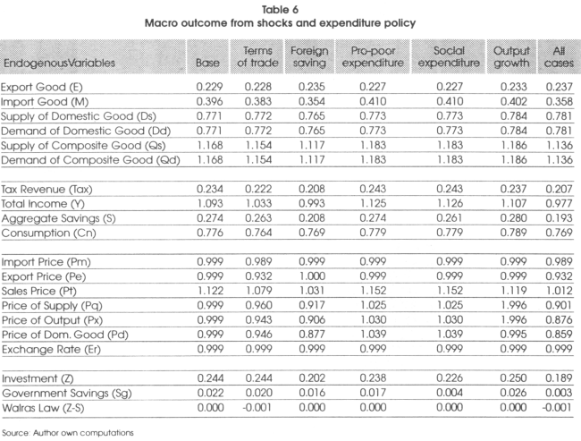
The full impact of the terms of trade shock results in a 1.5 per cent decrease in consumption and a 5.5 per cent decrease in total income compared to the base year. Also a 5.1 per cent decrease in tax revenues and 4 per cent decrease in aggregate savings, implying that without these last two happening, consumption would have decreased further. There is no observed change in investment. However, the drop of the domestic good price relative to the price of the export good and import good results in a 0.13 per cent increase in the production and consumption of the domestic good, a 0.4 per cent decrease in exports and 3.3 per cent decrease in imports.

The full impact of foreign savings flow reduction results in a 0.9 per cent decrease in consumption and a 9.1 per cent decrease in total income compared to the base year. Also an 11.1 per cent decrease in tax revenues and 24.1 per cent decrease in aggregate savings, implying that without these last two happening, consumption would have decreased further. There is also a 17.2 per cent decrease in investment. However, the drop of the export good price relative to the domestic and the drop of the domestic good price relative to the price of the import good results in a 0.77 per cent decrease in the production and consumption of the domestic good, a 2.62 per cent increase in exports and 10.6 per cent decrease in imports.

The full impact of social expenditure policy results in a 0.38 per cent increase in consumption and a 3 per cent increase in total income compared to the base year. Also a 3.8 per cent increase in tax revenues, 4.7 per cent decrease in aggregate savings and a 7.4 per cent decrease in investment. In the case of pro-poor expenditure alone there are some slight differences in that income increases a bit less, aggregate savings don't change and investment decreases less. However, in both cases the increase of the domestic good price relative to the price of the export good and import good results in a 0.2 per cent increase in the production and consumption of the domestic good, a 0.8 per cent decrease in exports and 3.5 per cent increase in imports. This last result shows that pro-poor expenditure and social expenditure in general conflicts with policies that promote exports and import substitution, that is, conflicts with policies that promote the production of tradables.

The full impact of output growth results in a 1.7 per cent increase in consumption and 1.3 per cent increase in total income compared to the base year. Also a 1.3 per cent increase in tax revenues, 2.2 per cent increase in aggregate savings and 2.4 per cent increase in investment. There is a drop of the domestic good price relative to the price of the export good and import good, however output growth increased production of the domestic and exports goods as well as demand of the import good, although with some differences. It results in a 1.7 per cent increase in the production and consumption of the domestic good, 1.7 per cent increase in exports and 1.5 per cent increase in imports.

Finally, the full impact of the combined effect of all cases simultaneously results in a 0.9 per cent decrease in consumption and 10.6 per cent decrease in total income compared to the base year. Also an 11.5 per cent decrease in tax revenues and 29.5 per cent decrease in aggregate savings, implying that without these two happening, consumption would have decreased further. There is also 22.5 per cent decrease in investment. However, the drop of the domestic good price relative to the price of the export good and import good results in a 1.3 per cent increase in the production and consumption of the domestic good, a 3.5 per cent increase in exports and 9.6 per cent decrease in imports.

A first conclusion is that under macroeconomic stability (no shocks and 1998 macro conditions) social expenditure policy would have had an important positive impact first on aggregate income and second on aggregate consumption and tax revenues, but negative impact on savings, investment and production of tradables.

A second conclusion is that the combined positive effects from social expenditure policy and low output growth on aggregate consumption, income and savings did not compensate the negative impacts from the combined terms of trade shock and reduction in foreign saving flows.

5.2 Experiments and poverty outcomes

The connection between the simple macro model and household welfare evaluation is based on the idea proposed by Devarajan and Go (2002). Households maximize an indirect utility function (v), which is a function of wages (w), profits (π) and prices (p). This indirect utility function is obtained from utility maximization as a function of net labor supply of households L and net commodity demand C, subject to the restriction that profits are the residual of commodity consumption expenditure pC minus labor income wL.

Differentiating this equation and applying Shephard's Lemma to observe the effects of small changes in prices, we obtain:

With the information on changes in income (wages and profits) and prices of the three goods given by the macro model, together with initial levels of labor income and commodity consumption given by the household surveys, the impact of shocks and macro policies on household welfare can now be computed.

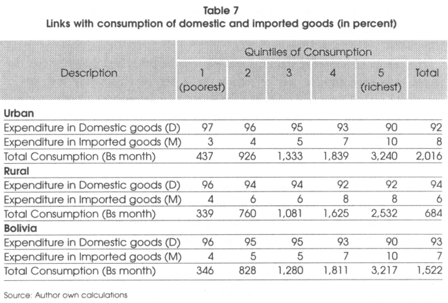
Aggregate consumption includes various items of food consumption and non-food consumption. Given that the definition of export (E), import (M) and domestic (D) goods have their origin in the input-output matrix, all items in the MECOVI survey were codified according to its respective row of the IOM. This procedure allows computing the household expenditure in terms of domestic and import goods, and gives the possibility to connect simulations of the 1-2-3 model (with changes in prices of the domestic and import goods) to each household, showing the effects on consumption after changes in these prices.

Table 7 shows the linking codes with consumption of domestic and imported goods.

The specific connection between the macro model and the household surveys is done through the use of an income multiplier and an expenditure multiplier. The income multiplier is simply the percent change in total income directly obtained from the simple macro model, but introduced to households only through labor income. The expenditure multiplier has two components, the expenditure multiplier for the domestic good (GHd) and the expenditure multiplier for the import good (GHm) Each of these components were computed the following way:

GHd₀₂ = Pd₀₂ Qd₀₂ = (Pd₉₈ + ΔPd_98-02) (Qd₉₈ + ΔQd_98-02) = Pd₉₈ Qd₉₈ + Pd₉₈ ΔPd_98-02 + ΔPd_98-02Qd₉₈ + ΔPd_98-02

Multiplier for d = GHd₀₂/GHd₉₈

GHm₀₂ = Pm₀₂ Qm₀₂ = (Pm₉₈ + ΔPm_98-02) (Qm₉₈ + ΔQm_98-02) = Pm₉₈ Qm₉₈ + Pm₉₈ ΔPm_98-02 + ΔPm_98-02 Qm₉₈ + ΔPm_98-02 ΔQm_98-02

Multiplier for m=GHm₀₂/ GHm₉₈

Where Pd and Pm are prices of the domestic good and import good respectively, obtained from the macro model. Qd and Qm are the quantities of the domestic and the import good respectively, also obtained from the macro model.

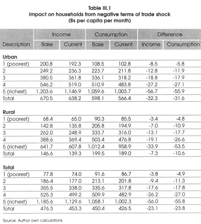
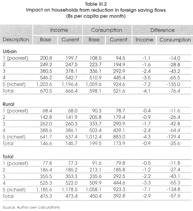
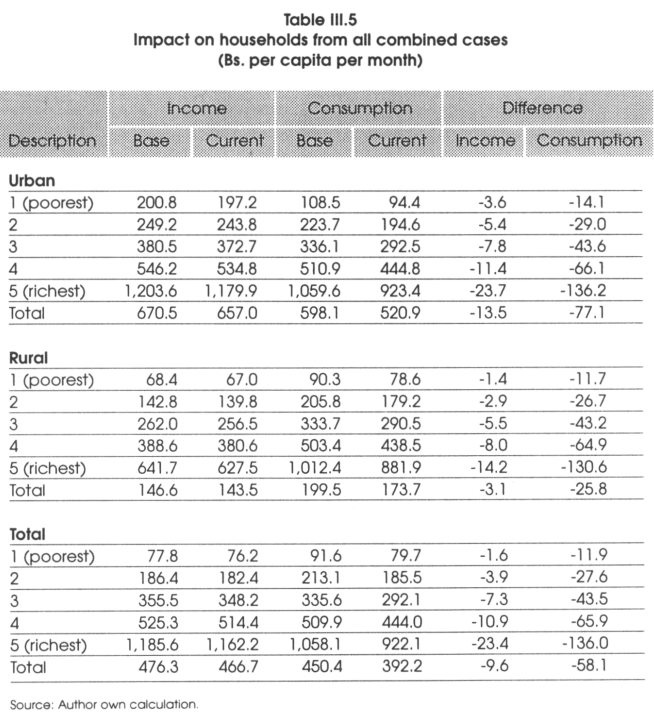
Table 8 shows the impact of shocks, expenditure policy and growth on household income and consumption by areas (Tables III.2 to III.5 in Appendix 3 show impact by quintiles). In the case of the terms of trade shock, people experiment loss of income by 4.8 per cent nationally and loss of consumption by 5.3 per cent nationally, and by similar percentages in both urban and rural areas. For the case of decreasing foreign saving flows, people experiment loss of income by 0.6 per cent nationally and loss of consumption by 12.8 per cent nationally, and by similar percentages in both urban and rural areas. Absolute losses of income and consumption are increasing the higher the income quintile and greater in urban areas, however, that is not necessarily the case in relative terms, for both negative shocks.

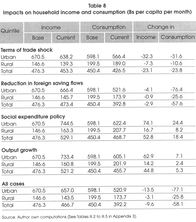
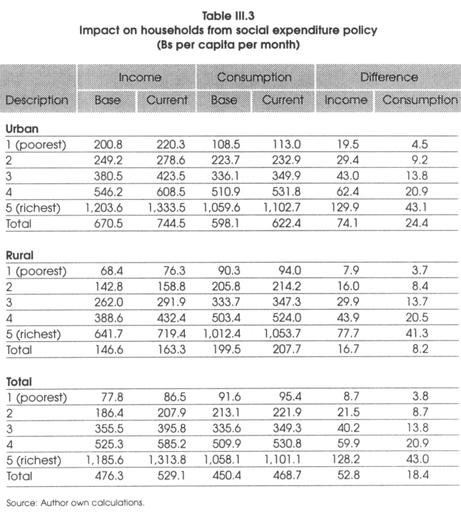
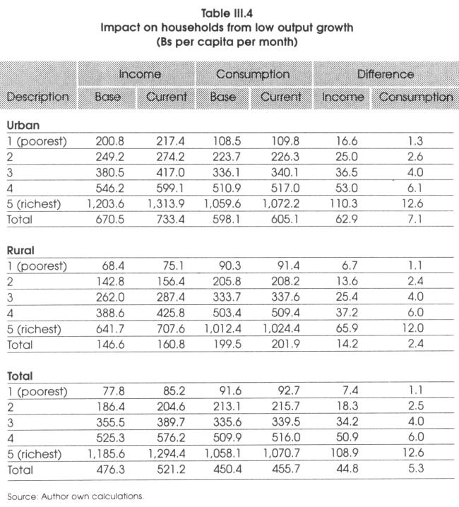
In the case of social expenditure policy, people experiment gains in income by 11 percent nationally and gains in consumption by 4 per cent nationally, and by similar percentages in both urban and rural areas. For the case of output growth, people experiment gains in income by 9.4 per cent nationally and gains in consumption by 1.2 per cent nationally, and by similar percentages in both urban and rural areas. Absolute gains of income and consumption are increasing the higher the income quintile and greater in urban areas, however, that is not necessarily the case in relative terms, for both positive shocks.

The combined impact of shocks, social expenditure policy and growth shows that people have experimented loss of income by 2 percent nationally and loss of consumption by 12.9 per cent nationally, and with similar percentages in both urban and rural areas. Absolute losses of income and consumption have increased the higher the income quintile and greater in urban areas, although that is not necessarily the case in relative terms.

One first conclusion from these experiments comes from comparing the magnitudes of the differential effects on household income and consumption levels by quintiles and areas. The negative effect on income has been greater from the terms of trade shock and the negative effect consumption has been greater from reduction in foreign saving flows.

A second conclusion is that under macroeconomic stability (no shocks and 1998 macro conditions), social expenditure policy would have had an important positive impact first on household income and second on household consumption by quintiles and areas.

A third conclusion is positive effects from the combined social expenditure policy and low output growth on income and consumption, did not compensate the negative impacts from the combined terms of trade shock and foreign saving reduction.

Table 9 shows the impact of shocks, expenditure policy and low growth on poverty measures expressed in the FGT indicators. The terms of trade shock increases the number of poor by an average of 1.1 percent nationally, more in urban areas then in rural areas. Poverty gap decreases nationally by 0.2 per cent and poverty intensity decreases nationally by 0.1 per cent. The negative change of the poverty gap and poverty intensity percentages nationally is explained by the effect of the new poor, who would usually be the ones that were just above the poverty line and who would require less additional income to recover its previous welfare position. By areas the poverty gap and poverty intensity decreases in urban areas but increases in rural areas.

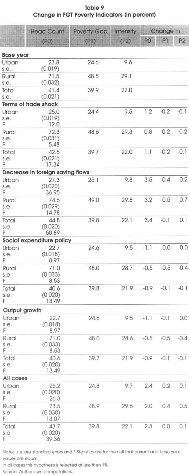
The foreign saving flow reduction increases the number of poor by an average of 3.4 per cent nationally, more in urban areas then in rural areas. Poverty gap decreases nationally by 0.1 per cent and poverty intensity increases nationally by 0.1 per cent. The negative change in the poverty gap percent nationally is again explained by the characteristics of the new poor. However, the poverty gap and poverty intensity increases in both urban and rural areas when calculating them separately, more so in rural areas in both cases.

The social expenditure policy decreases the number of poor by an average of 0.9 per cent nationally, more in urban areas (1.1 per cent) then in rural areas (0.5 per cent). The poverty gap and poverty intensity would also decrease nationally by 0.1 per cent, explained fully by their decrease in rural areas.

Similarly, the low output growth decreases the number of poor by an average of 0.9 per cent nationally, more in urban areas (1.1 per cent) then in rural areas (0.5 per cent). The poverty gap and poverty intensity would also decrease nationally by 0.1 per cent, mostly explained by its decrease in rural areas in the first case and explained fully by its decrease in rural areas in the second case.

The combined effect of shock, expenditure policy and low output growth have increased the number of poor by an average of 2.3 per cent nationally, more in urban areas (2.4 per cent) then in rural areas (2 per cent). The combined effect does not show an effect on the poverty gap when measured nationally, but it shows an increase in urban and rural areas when measured separately, more so in rural areas (0.4 per cent) then in urban areas (0.2 per cent). The combined effect shows an increase in poverty intensity by 0.1 per cent nationally and also by areas, more so in rural areas (0.5 per cent) then in urban areas (0.1 per cent).

A first conclusion is that poverty increases, measured by the head count ratio, has been greater from reduction in foreign savings flows then from the terms of trade shock. Poverty increases, measured by the poverty gap and poverty intensity is concentrated in rural areas, and has been greater from the impact of reduction in foreign saving flows then from the terms of trade shock.

A second conclusion is that under macroeconomic stability social expenditure policy would have had an important impact in reducing the number of poor nationally, more in urban areas then in rural areas. It would have also reduce the poverty gap and poverty intensity in both areas, although more so in rural areas.

A third conclusion is that the combined positive effects from poverty reduction through social expenditure policy in an environment of low output growth, did not compensate the negative impacts on all measures of poverty from the combined terms of trade shock and reduction in foreign saving flows.

Given the diverse characteristics of the Bolivian population, captured by the 1999 survey, we can know which groups were impacted the most and by what magnitude. This information is presented in Table 10 based on the combined effects of shocks, expenditure policy and low growth on poverty. The number of poor increased the most in the age group of 19-30 nationally and in urban areas. In rural areas the most affected were in the age group of 31-45. In terms of sex, the number of poor increased the most among males, nationally and in both urban and rural areas.

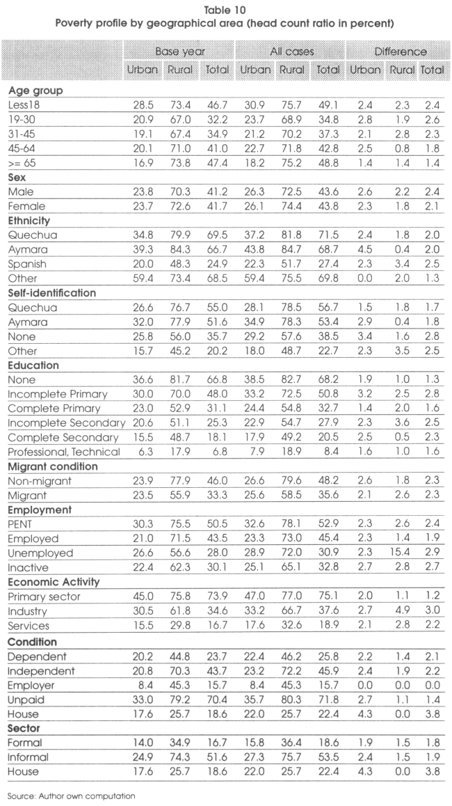
When analyzing the increase in the number of poor by ethnicity, the classified as Spanish were impacted the most nationally and secondly the Aymara and Quechua equally. In rural areas the most affected were also the classified as Spanish and secondly the classified as "other". In urban areas the number of poor increased the most among the Aymara and secondly among the Quechua and Spanish. By self-identification, the number of poor increased the most under the classification of "none" Quechua or Aymara, nationally and in urban areas, being second the self-identified as "other" and Aymara. In contrast, in rural areas the number of poor increased the most under the self-identification of "other".

In terms of education, first those with incomplete primary education were affected the most nationally and in urban areas, increasing the number of poor. Second was the population with complete or incomplete secondary education. In rural areas the number of poor increased the most first among those with an incomplete secondary education and second among those with complete or incomplete primary education.

In terms of employment, the number of poor increased the most among the unemployed nationally and in rural areas, secondly the inactive and those not in working age (PENT). In the case of rural areas the number of poor increased by 15.4 per cent among the unemployed. In urban areas the number of poor increased the most first among the inactive and second among all other employment classification equally.

By economic activity, the number of poor increased the most in the industry sector, nationally and in both urban and rural areas. By economic condition and by sector, the number of poor increased the most in the classification of "house" (house work), nationally and in urban areas. In rural areas, the number of poor increased the most when "independent" and when "formal" or "informal".

 

6. Conclusions and policy implications

Shocks and poverty reduction policy were analyzed individually and jointly in an environment of low growth in an effort to simulate the actual experience of the Bolivian economy during the period 1998-2002. The analytical method was based in the connection of a simple macro model of the 1-2-3 type with household data (Devarajan and Go, 2002). Analysis was made in terms of the direction and order of magnitude of the differential effects of shocks and policy on i) macro aggregate consumption, income, saving and prices, ii) on income and consumption levels of households, and iii) on poverty measures.

There following are some methodological limitations:

1.   Pro-poor government expenditure in education, health and infrastructure for development will have its full returns in terms of poverty reduction only in the long run. Therefore what we measure here is only the short run effects of government expenditures, believing that these expenditures will have a short run effect on overall household income and expenditures.

2.   Given that the distribution of income and consumption by quintiles is based on a fixed year (1999), which are applied to overall changes in household income and consumption, then this methodology cannot simulate the more complicated process of income and consumption redistribution.

3. Given that the 1-2-3 model is built on highly aggregate macroeconomic data, then this model cannot simulate the more complicated process of resource distribution by economic sectors and its consequent effects on household income and expenditures.

The following are some conclusions and implications.

1.   The terms of trade shock experienced by the Bolivian economy had a greater negative impact on household income then the experienced reduction in foreign saving flows. At the same time, reduction in foreign saving flows had greater negative impact on household consumption then the terms of trade shock.

2.   Poverty increase measured by the head count ratio has been greater from reduction in foreign saving flows then from the terms of trade shock. Poverty increase measured by the poverty gap and poverty intensity has concentrated in rural areas, and has also being greater from reduction in foreign saving flows then from the terms of trade shock.

3.   Under macroeconomic stability (no shocks and 1998 macro conditions) social expenditure policy for poverty reduction would have had an important positive impact on aggregate income, consumption and saving, on household income and consumption levels (more so in income then consumption), in reducing the number of poor (more in urban then rural areas), and in reducing poverty gap and poverty intensity (more so in rural areas).

4.   The combined positive effects from social expenditure policy in an environment of low output growth, did not compensate the combined negative impacts from the terms of trade shock and reduction in foreign saving flows.

These conclusions show that under macroeconomic disequilibrium poverty reduction efforts become policies of poverty containment or safety net programs during a period of economic recession. They also show that if poverty reduction is seen as a long term objective, particularly in a country that is starting at high poverty levels, then commitment to long term macroeconomic stability must be a key general policy. It also suggests that this general policy must be accompanied by policies directed at ensuring positive growth under disequilibrium, given that the economy will certainly experiment other episodes of shocks in the medium and long term.

The paper also shows that the magnitude of poverty reduction effort does matter. If effort produces small positive effects compared to large negative effects of shocks, then poverty reduction policy is not real. If effort actually produces larger positive effects compared to negative effects of shocks, then poverty reduction policy may be real. However, if effort is larger, the macro analysis warns of other macroeconomic effects from social expenditures policies for poverty reduction, those of export decreases, import increases and investment decreases.

Bolivia probably doesn't have the financial resources for a greater scale poverty reduction effort. If this is the case, then a more effective way to avoid welfare looses and maximize poverty reduction is to defend macroeconomic stability. This implies work on preparing for external shocks and on structural aspects of the economy, like greater export and trade diversification and large improvements in domestic productivity.

 

Notes

* The original version of this study has been prepared for the Global Development Network (GDN) Project on Macroeconomic Policy Challenges of Low Income Countries. The authors would like to acknowledge comments from Raimundo Soto to this paper and its earlier version. Errors are our own. The authors gratefully acknowledge the financial support from GDN as well as its administrative support through Gary McMahon.

**	Gover Barja Daza: Maestrias para el Desarrollo. Javier Monterrey Arce: National Institute of Statistics. Sergio Villarroel Bohrt: Ministry of Economic Development.

1   Private domestic investment was approximated by subtracting public investment and FDI from the economy's gross fixed capital formation plus inventory variations.

2   The extended version adopted in the current study (based on Devarajan. Lewis and Robinson, 1990 and Devarajan et al 1997). includes government revenues and expenditures, savings, and investment, in order to consider policy instruments that are used to adjust macroeconomic imbalances.

3   This study uses the Adult Equivalt Scale computed by the Organization for Economic Cooperation and Development (OECD), recommended by the World Bank (2003) and defined as: AES = 1 +07(adults-1 )+0.5children. The equation reflects a parametric scale as function of the relative needs of the household members. Interpreting its functional form, AES has a value of 1 with the first adult, every additional adult is equivalent to 0.7 of the first adult, and each child is equivalent to 0.5 of the first adult.

4   INE defines urban as those cities with populations greater then 2000. This definition has been critized in that it may underestimate the weight of rural areas.

5   The two main characteristics of the CES/CET functions are: i) they are homogeneous of degree one (linearly homogeneous); and ii) they have a constant elasticity of substitution.

6   See Appendix 1 tor detailed mathematical procedure.

7   The composite good price P^x corresponds to GDP deflator.

8    The composite good price P^q corresponds to an aggregate consumer price or cost-of -living index.

9   The equilibrium conditions are not all independent. To prove this, it suffices to show that the model satisfies Walras's Law.

10   Each cell represents a payment from a column account to a recipient in a row account.

11   According to equation 5.

14   Note that in the Bolivian economy there are no export subsidies.

15   Note that all income is spent on the single composite good.

 

REFERENCES

Andersen, Lykke. 2003. "Baja movilidad social en Bolivia: causas y consecuencias para el desarrollo". Latin American Journal for Economic Development: No. 1, September 2003. IISEC, Universidad Católica Boliviana.

Barja, Gover, David McKenzie and Miguel Urquiola. 2004. "Capitalization and privatization in Bolivia: An approximation to an evaluation". In: John Nellis y Nancy Birdsall (editors). Reality Check: Assessing the Distributional Impact of Privatization. Washington DC: The Center of Global Development Publisher. Forthcoming.

Barja, Gover and Miguel Urquiola. 2003. "Capitalization, regulation and the poor: access to basic services in Bolivia". In: Catherine Waddams Price y Cecilia Ugaz (editors). Utility Privatization and Regulation: A fair deal for consumers? The World Institute for Development Economics Research. Edward Elgar Publishing. UK.

Barja, Gover, Javier Monterrey and Sergio Villarroel. 2003. "The elasticity of substitution in demand for non-tradables goods in Bolivia". The Latin American and Caribbean Research Network, IADB.

Deaton, Angus and Zaidi Salman. 2002. "Guidelines for constructing consumption aggregates for welfare analysis. Living Standard Measurement Study". Working paper N° 135. World Bank. Washington. U.S.A.

Deaton, Angus. 1997. "The analysis of household surveys: A microeconometric approach to development policy". The Johns Hopkins University Press. U.S.A.

Devarajan, Shantayanan and Delfin S. Go. 2002. "The 123PRSP Model" In: Techniques and Tools for Evaluating the Poverty Impact of Economic Policy, Chapter 13, World Bank.

Devarajan, Shantayanan, Jeffrey D. Lewis, and Sherman Robinson. 1990. "Policy Lessons From Two-sector Models". Journal of Policy Modeling. 12 (4): 625-657.

Devarajan, Shantayanan, Go Delfin S., Lewis Jeffrey D., Robinson Sherman and Sinko Pekka. 1997. "Simple General Equilibrium Modeling". In Joseph Francois and Kenneth Reinert (eds), Applied Methods/or Trade Policy Analysis: A Handbook. Cambridge: Cambridge University Press.

Devarajan, Shantayanan, Jeffrey D. Lewis, and Sherman Robinson. 1993. "External Shocks, Purchasing Parity Power and The Equilibrium Real Exchange Rate". World Bank Economic Review 7:45-63.

Engle, R.F. and C.W.J. Granger. 1987. "Cointerpretation and correction. Representation, estimation and testing". Econometrica. 55, 251-276.

Foster James, Greer Joel and Thorbecke Erik. 1984. "A class of decomposable poverty measures". Econometrica. Vol. 52. Issue 3. 761-766..

Garron, Mauricio, Katherina Capra and Carlos Machicado. 2003. "Privatization in Bolivia: the impact of firm performance". The Latin American and Caribbean Research Network, IADB.

Hylleberg, S., R. F. Engle, C. W.J. Granger, and B.S. Yoo. 1990. "Seasonal Interpretation on Cointegration". Journal of Econometrics. 44 (2), 215-238.

Jemio, Luis Carlos and Manfred Wiebelt. 2001. "¿Existe espacio para políticas anti-shocks en Bolivia?" Latin American Journal of Economic Development: N° 1, September 2003. MSEC, Universidad Católica Boliviana.

Lanjouw, Jean Olson and Lanjouw Peter. 1997. "Poverty Comparisons with non-compatible data". Policy Research Working Paper 1709. World Bank. Washington.

Medina, Fernando. 2002. "Equivalence Scales: A brief review of concepts and methods". Economic Commission for Latin America and the Caribbean. Third Meeting of the Expert Group on Poverty Statistics (Rio Group). Lisbon.

Republic of Bolivia. 2001. "Poverty Reduction Strategy Paper" (PRSP).

Republic of Bolivia. INE and United Nations. 2003. "Bolivia: Social and Demographic Characteristic of Indigenous People".

Republic of Bolivia. INE, UDAPE and World Bank. 2003. "Poverty and Inequity by Bolivian Municipal areas: Estimation of Consumption Expenditure by Combining the 2001 Census and Household Surveys".

Republic of Bolivia. Unidad de Análisis de Políticas Sociales y Económicas. 2003. "Estrategia Boliviana de Reducción de la Pobreza: Informe de Avance y Perspectivas".

Sen, Amartya. 1976. "Poverty an ordinal approach to measurement". Econometrica. Vol. 44. Issue 2. pages 219 - 231.

Spatz, Julius. 2003. "The impact of structural reform on wages and employment: the case of formal versus informal workers in Bolivia". Latin American Journal of Economic Development. N°.2, April 2004. MSEC, Universidad Católica Boliviana.

Steward, Frances. 2003. "The implications for chronic poverty of alternative approaches to conceptualizing poverty". Department of Financial International Development (DFID). England.

Thiele, Rainier and Manfred Wiebelt. 2003. "Attacking poverty in Bolivia. Past evidence and future prospects: Lessons from a CGE analysis". Working Paper 6/2003, IISEC, Universidad Catolica Boliviana.

World Bank. 2003. Poverty Manual. Washington. U.S.A.

 

Appendix 1

Description of the 1-2-3 model

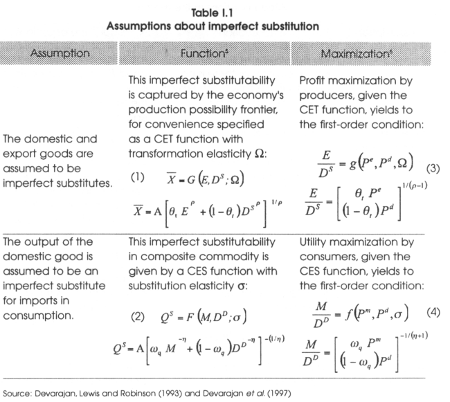
Aside from Equations (1), (2), (3), and (4) showed in Table I.1. equation (5) is part of the "real flows" side of the model, which defines total demand for the composite good (absorption) showing that the value of the goods demanded must equal aggregate expenditure:

In Equation (5), C represents aggregate consumption, Z represents aggregate real investment and is the real government demand.

Complementing the information presented in Table I.2, two additional price equations are introduced: i) one that considers the sales price of composite goods P^t when indirect taxes (t^s) are added to the price of the composite good (P^q); and ii) a numeraire price, in this case the nominal exchange rate R, since only relative prices matters:

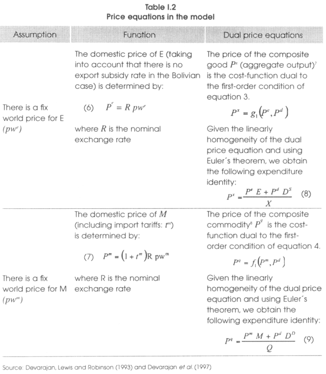
Regarding the market-clearing equilibrium conditions', supply must equal demand for "D" and "Q" (Equations 12 and 13 respectively), the balance-of-trade constraint must be satisfied adjusting grants (ft) and remittances (re) from abroad (Equation 14), and also the government-budget constraint (public savings) must be considered as the residual of tax revenue (T) plus foreign grants less government consumption () and transfers (tr) to households (Equation 15).

The income flows (nominal flows) among the actors in the economy can be tabulated in a social account matrix (SAM) with six accounts: one for each actor, a "capital" account that reflects the saving-investment balance, and a "commodity" account that keeps track of absorption. Table I.3 presents this social account matrix.

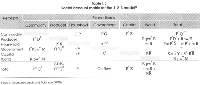
Four equations can be extracted from the information presented in Table I.3; Equation (16) that corresponds to household income "Y" (sum of 3^rd row). Equation (17) determining government revenue "T " (sum of the 4^th row: T = t''' R pw''' M + t^s P^q Q^D + t^yY, Equation (18) representing total savings "S"', and finally Equation (19) that determines aggregate household consumption "C" The latter can be obtained rearranging terms of the 3^rd column¹⁵ and takes the following form:

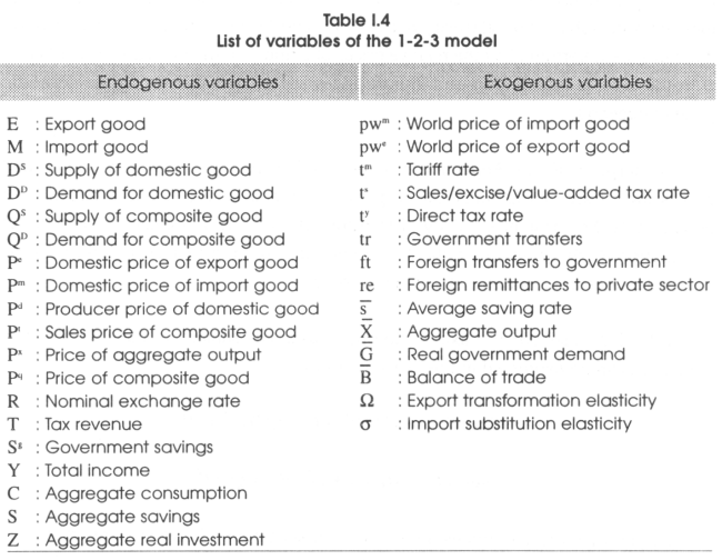
Summarizing, the full analytical model is a system of nineteen equations with nineteen endogenous variables. Endogenous and exogenous variables are listed below:

 

Appendix 2

Econometric Procedure and Elasticity Estimation

1. Methodology and data source

The 123 macro model divides the economy into two sectors (tradable (E + M) and non-tradable (D)) and three goods markets (export good E, domestic good D and import good M). In this economy the production possibilities frontier is specified as a constant elasticity of transformation (CET) function with transformation elasticity between E and D^s. Utility in consumption is specified as a constant elasticity of substitution (CES) function with substitution elasticity between D^D and M. Production and consumption decisions are determined by the relative prices of E and D in the first case and of M and D in the second case. Export and import prices are exogenous making the domestic price endogenous.

The purpose of this Appendix is to present the methodology, data source and processing, study of the statistical properties of the data and finally production of estimates of the constant elasticity of transformation (CET) and constant elasticity of substitution (CES), required for the 123 model. It is desired that estimation of these parameters best represent the Bolivian economy.

In the CES case, utility maximization by households subject to a standard budget constraint can be expressed in the following form:

The parameter η determines the elasticity of substitution between consumption of the import good and consumption of the domestic good, which is given by v = 1/(1+η) for -∞< η <+1, w is the share parameter, P^k is the price of the import good, P^D is the price of the domestic good, Q^S *P^Q is a budget constraint expressed in terms of the composite good and t is time. Solution of the maximization problem yields the following optimality condition for the allocation of consumption:

This condition reduces to the following log-linear testable relationship:

In the CET case, maximization of aggregate production subject to a constant elasticity of transformation function can be expressed in the following form:

The parameter p determines the elasticity of transformation between the production of the export good and the domestic good, which is given by u = 1/(p-1) for 1< p <+∞, θ is the share parameter, P^E is the price of the export good, P^S is the price of the domestic good, X°*P^X is the value of aggregate product X° which is fixed. Solution of the maximization problem yields the following optimality condition for the allocation of production:

This condition reduces to the following log-linear testable relationship:

Both testable relationships based on the CET and CES functions describe a long run equilibrium condition, therefore it is of interest to estimate a cointegrating relationship among the variables. In the first case the elasticity corresponds to the long-run equilibrium relationship between the production ratio and the price ratio of the export good relative to the domestic good. In the second case the elasticity corresponds to the long-run relationship between the consumption ratio and the price ratio of the import good relative to the domestic good. In each case the price ratio describes an internal real exchange rate, in the first case it is a production exchange rate (depreciation is an incentive for exports) and in the second it is a consumption exchange rate (depreciation is an incentive for imports).

The source for the data is the national accounts statistics produced by the Bolivian National Institute of Statistics (INE). INE produces national accounts data on a quarterly basis and time series for all of its components are available from the first quarter of 1990 to the second quarter of 2004 (the last two quarters are preliminary), in nominal and real terms (base 1990). The time series required for the study must be consistent with an economy that produces two goods (one export and one domestic) and demands two goods (one import and one domestic). For the elasticity of substitution in supply (CET function) we need the quarterly time series of the export good (EE), domestic good (DCK), price of the export good (PE) and price of the domestic good (PD). For the elasticity of substitution in demand (CES function) we need the time series of the import good (MCK), domestic good (DCK), price of the import good (PM) and price of the domestic good (PD). All of these can be obtained from the national accounts with the following processing:

EE            = no processing required.

MCK         = Total imports MM - intermediate imports and raw materials.

DCK          = Total household demand + total government demand + total investment-MCK.

PE            = Nominal EE / Real EE

PM            = Nominal MCK / Real MCK

PD            = Nominal DCK / Real DCK

EE/DCK     = Ratio of export good production to domestic good production.

PE/PD        = Ratio of the export good price to the domestic good price.

MCK/DCK  = Ratio of import good consumption to domestic good consumption.

PM/PD       = Ratio of the import good price to the domestic good price.

 

2. Statistical properties of the data

The following figures present the raw quarterly time series of interest, where ED = EE/DCK is the real production ratio of the export good relative to domestic good, PED = PE/PD is the price ratio of the export good relative to the domestic good, MD = MCK/DCK is the real consumption ratio of the import good relative to the domestic good and PMD = PM/PD is the price ratio of the import good relative to the domestic good.

 

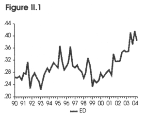
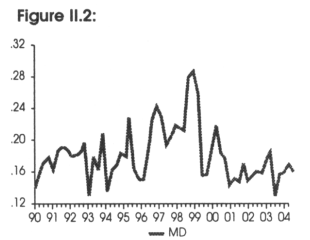
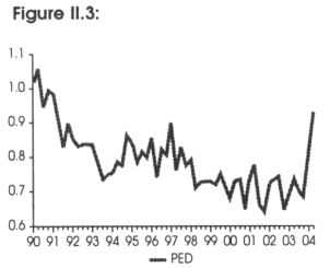
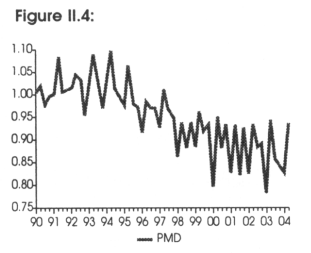
Table II.1 presents the standard ADF test applied to the data in levels, indicating the variables LED = log(ED), LMD = log(MD), LPED = log(PED) and LPMD = log(PMD) are all non-stationary under different test specifications.

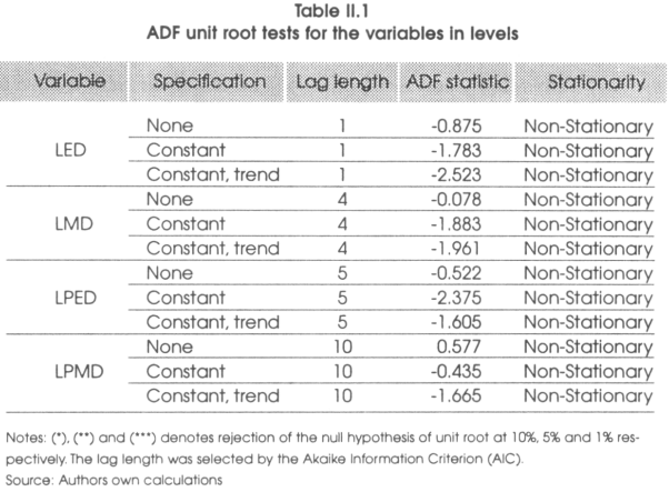
Table II.2 presents the standard ADF test applied to the data in first difference, indicating the first difference of LED and LMD are stationary under different test specifications. The first difference of LPED is also stationary except when a constant and trend are included in the test specification. The first difference of LPMD is stationary only when a constant is included in the test specification.

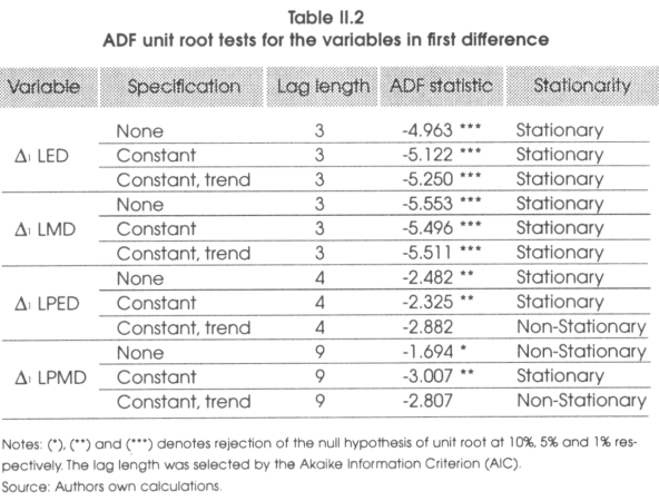
Comparing Table II. 1 and II.2 it is possible to conclude that the variables LED and LMD are integrated of first order or I(1). The variable LPED is not I(1) only when the test includes constant plus trend. The variable LPMD is I(1) only when the test includes a constant.

Traditional unit root and co-integration tests were developed for non-seasonal or zero frequency data, which could also be applied to quarterly data only if it is proven that unit roots at other frequencies are not present (half frequency or biannual unit root and one fourth frequency of annual unit root). It is important to notice that the elasticity of interest in this study corresponds to the long run equilibrium relationship between LED and LPED and between LMD and LPMD, that is, it is strictly a non-seasonal or zero frequency relationship in the data.

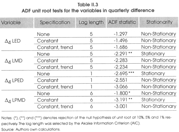
Seasonal differencing is often used to remove non-stationarity in seasonal data. In this case the quarterly difference operator is Δ₄y_t = y_t- y_t-4. Table II.3 presents the ADF test applied to the quarterly difference of the data. Results show that the quarterly difference of LED is non-stationary under any test specification, which supports the result that this variable is I(1). The quarterly differences of LMD and of LPED are stationary only when no deterministic variables are included in the test specification. The quarterly difference of LPMD is stationary only when a constant is included in the test specification. Stationarity of the quarterly difference implies that the time series may contain either a non-seasonal unit root, a biannual unit root, an annual unit root, or a combination of these types of unit roots.

The HEGY procedure introduced by Hylleberg et al. (1990) is appropriate to find out which types of unit roots are contained in the data. The quarterly difference operator Δ₄=(I-L⁴) can be decomposed as, (I-L⁴) = (I-L)(I+L)(I+L²) = (I-L)(I+L+L²+L³), which has four roots, one at zero frequency, one at two cycles per year and two complex pairs at one cycle per year. The HEGY procedure consists in the following testable regression model, which can be estimated by OLS.

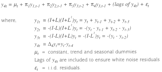
Based on the HEGY regression the following hypothesis can be tested using critical values computed by Hylleberg et al. (1990):

H_A: π₁ = 0 or non-seasonal unit root
H_B:π₂ = 0 or biannual unit root
H_c: π₃ = π₄ = 0 or annual unit root

Table II.4 presents estimated statistics from application of the HEGY regression to the data. In the case of LED there is consistent rejection of H_B and H_C and failure to reject H_A implying unit root only at zero frequency (non-seasonal unit root), that is, the variable must be I(1). This result supports the previous finding.

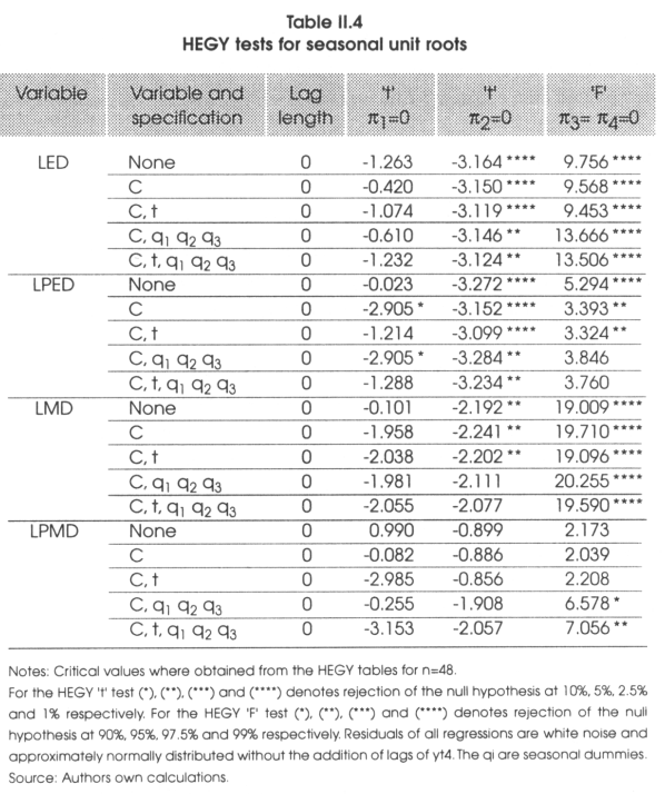
In the case of LPED and LMD there is consistent rejection of H_B and H_C and failure to reject H_A when no seasonal dummies are included in the test specification. That is, LPED and LMD are I(1) as found before as long as no seasonal dummies are included in any regression procedure.

In the case of LPMD there is consistent failure to reject H_A, H_B and H_C implying unit root at all frequencies (consistent with earlier findings). This result suggests that for LPMD there is need to filter out the unit root components other then the one of interest at zero frequency, this way the new LPMD, say LPMD1, would be I(1). The filter to remove the seasonal roots would be the following, where y_1t is the filtered series already computed above: (I-L⁴)/(I-L)y_t = (I+L+L²+L³)y_t = y_1t.

 

3. Co-integration test

The issue is to find weather the variables of interest are co integrated, that is if there is a linear combination of the pair of variables LMD and LPMD1 and the pair of variables LED and LPED that is stationary. If these pairs of variables are co integrated, then the linear combination would express the long term relationship among them.

Engle and Granger (1987) proposed a two-step estimator for models involving co-integrated variables. In the first step, the co-integrating parameters are estimated by running a static regression in the levels of the variables. In the second step, these are used in estimating an error correction model. Both steps require only OLS. The first step is our main interest here, in testing whether the residuals of the estimated regression in levels produces a stationary time series. The following are the estimated co-integrating equations:

CET co-integrating equation:

log(E/D) = (-1.38 + 0.01 t-0.18 dcrisis) + 0.248 log(PE/PD) + Res1

CES co-integrating equation:

log(M/D) = (-1.61 - 0.004 t - 0.37 dcrisis) - 0.81 log(PM/PD) + Res2

where t is time and dcrisis is a dummy variable that captures the shift during the current period of economic crisis, taking a value of 1 from the first quarter of 1999 to the second quarter of 2004 and 0 otherwise. Res1 and Res2 are the residuals of the estimated equations.

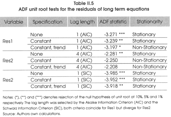
Table II.5 presents the standard ADF test applied to the estimated residuals of the co-integrating equations. Results show evidence of stationarity for Res1 when no deterministic variables are included or when only a constant is included in the test specification. Results also show consistent evidence of stationarity for Res2 under any deterministic specification of the test with one lag. There is also evidence of stationarity for Res2 when no deterministic variables are included in the test specification with four lags.

The CET co-integrating equation suggests on average an elasticity of substitution of 0.248 in the production of the export good relative to the domestic good when there is a change in their relative prices. In addition the positive sign indicates that, when the price of the export good increases while the price of the domestic good remains constant, the production of the export good will increase and the production of the domestic good will decrease. Result in accordance to theory.

The CES co-integrating equation suggests on average an elasticity of substitution of 0.81 in the consumption of the import good relative to the domestic good when there is a change in their relative prices. In addition the negative sign indicates that, when the price of the import good increases while the price of the domestic good remains constant, the consumption of the import good will decrease and the consumption of the domestic good will increase. Result in accordance to theory.

Although both estimated co-integrating parameters are inelastic, the CET parameter is more inelastic compared to the CES parameter, implying that producers are much slower to react to price changes (probably due to structural rigidities) compared to consumers.

The following are the corresponding error correction models (ECM) or second step of the Engle and Granger estimation procedure, where ε1_t and ε2_t are white noise residuals.

CET ECM:	Δlog(E/D)t = 0.006 - 0.44 Res1t-1 + ε1t t-Stat: (0.46) (-3.64) R2 = 0.19 Skewness = -0.45 Kurtosis = 4.37
CES ECM:	Δlog(M/D)t = -0.0002 - 0.32 Δ log(M/D)t-3 - 0.65 Res2t-1 + ε2t t-Stat: (-0.01)(-3.26)(-5.56) R2 = 0.50 Skewness = -0.46 Kurtosis = 3.94

 

Appendix 3

Household Tables