


Servicios Personalizados
Revista
Articulo
 Inglés (pdf)
 Articulo en XML
 Referencias del artículo
 Enviar articulo por email
Indicadores
-
 Citado por SciELO
 -
 Accesos
Links relacionados
-
 Similares en
SciELO
Similares en
SciELO
Compartir

 Permalink
Revista Latinoamericana de Desarrollo Económico
versión impresa ISSN 2074-4706versión On-line ISSN 2309-9038
rlde n.4 La Paz abr. 2005
TRABAJO DE INVESTIGACIÓN
Empirical Investigation of the Effects of the Fundamentals on the Exchange Rate
Juan R. Castro*
Summary
This paper examines, by using several econometric techniques, the effects of foreign reserves and other fundamental variables on the exchange rate using the target zone theory. This paper uses monthly data for Chile from January 1979 to November 1 997. The data used consists of foreign reserves, credit from the Central Bank, domestic reserves, imports, exports, claims on government, GDP, foreign liabilities, domestic and foreign interest rate. We find that the interest differential does not have any effect on depreciation, rejecting the target zone implication that the domestic interest rate can be used to manage the exchange rate. We find that foreign reserves support the exchange rate by reducing the exchange rate depreciation, and the exchange rate and foreign reserves follow a negative relationship, which supports the assumption that increasing the foreign reserves appreciates the exchange rate.
Resumen
Este documento de investigación examina, utilizando varias técnicas de econometría, los efectos de reservas extranjeras y otras variables fundamentales en la tasa de cambio que utiliza la teoría de la zona de bandas. Para ello utiliza datos mensuales de Chile desde enero 1979 hasta noviembre 1997. Los datos utilizados consisten en reservas extranjeras, el crédito del Banco Central, las reservas domésticas, las importaciones, las exportaciones, los reclamos en el Gobierno, el PIB, las obligaciones extranjeras y el tipo de interés domestico y extranjero. Encontramos que la diferencia de las tasas de interés no tiene ningún efecto en la depreciación, rechazando la implicación de la zona de bandas por el que el tipo de interés doméstico se puede utilizar para manejar la tasa de cambio. Encontramos que las reservas extranjeras sostienen la tasa de cambio reduciendo la depreciación de la tasa de cambio, y la tasa de cambio y las reservas extranjeras siguen una relacion negativa, que sostiene la teoría de que aumentando las reservas extranjeras aprecian la tasa de cambio.
1. Introduction
The existing literature on emerging foreign exchange markets has dealt with the problems associated with exchange rate fluctuations and currency devaluations.1 In this paper we investigate the effects of foreign reserves and fundamental variables on the exchange rate in Chile by employing the target zone model of Krugman (1991). Existing literature has tested the theory of target zone mainly by using the data from European countries.2 Several countries from Latin America and Asia have also used a policy of target bands on their exchange rates, which are similar to the bands established by the European Monetary System.
Chile is a good case for applying the model because it has been using a managed exchange rate policy since the mid-1980's, and its government has introduced a nominal exchange rate system. A crawling band characterizes this system, which is similar to the European target bands. While developed markets, such as many European countries, employ domestic money supply as one of the fundamentals to manage exchange rates, emerging markets tend to use foreign reserves as the primary tool to manage their currencies. Therefore, it is appropriate to treat foreign reserves as an important variable to maintain the targeted exchange parity rate.
In their model, Krugman and Miller (1991) emphasize altering the relationship between the fundamentals (i.e., interest rates, reserve ratios, terms of trade and other variables) and exchange rate by changing the money supply. Many emerging markets manage their exchange rates by using foreign reserves rather than domestic currency.3 The majority of these countries even industrialized countries such as Japan) use foreign reserves to counterattack any change in the fundamentals that might cause unwanted movements in the exchange rates.4
In general, most emerging countries use foreign reserve criterion to maintain exchange rate parity conditions and to counterattack the speculative attacks by sustaining constant domestic money supply and changing the supply of foreign reserves according to the demand. The monetary authority must have enough reserves to support any given increase in foreign reserve demand and prevent speculative attacks. Although the relationship between the reserve ratios and the exchange rate will differ from country to country, less developed countries should have higher demand for foreign reserves due to less market efficiency, high exchange rate volatility, poor monetary credibility and other factors.
The objectives of this research are as follows: first we show how a basic target zone model can be used to analyze the effects of the ratio between foreign reserves and domestic credit on the exchange rate by using a system of equations; second, we test these equations by using different quantitative approaches using data from Chile and compare the estimated points with the actual ratios and third, we study the effects of the different fundamentals on the Chilean exchange rate.
This paper is organized as follows: target zone model is presented in Section 2, a system of equations is derived in Section 3, methodology is presented in Section 4, the data is presented in Section 5, statistics are provided in Section 6, effects of the fundamental variables over the exchange rate, using instrumental variables, are discussed in Section 6, effects of the fundamentals on the exchange rate, using a vector auto regression, are examined in Section 7 and, finally Section 8 presents the conclusions.
2. Target Zone Model
The standard target zone model has two crucial assumptions. First, the exchange rate target zone is perfectly credible; market agents believe that the Central Bank will maintain the exchange rates within the specified bands. Second, the target zone will only be defended with marginal interventions; no interventions exist as long as the exchange rates are in the interior of the exchange rate bands. The current paper closely follows a model presented by Krugman and Miller (1991) and focuses on the ratios among the foreign reserves and other fundamental variables.
The basic target zone model is:
where s(t) is the exchange rate defined as the value of one U.S. dollar in terms of Chilean pesos (Peso/US$) and f(t) denotes fundamental composite exogenous shocks (i.e. imports, exports, foreign debt, domestic credit, GDP, foreign and domestic interest rates and other macro variables). The coefficient α is the semi-elasticity of money demand with respect to home interest rate, and E[ds/dt] is the expected change in the exchange rate. Assume that a composite exogenous shock follows a random walk:5
where σ is the standard deviation and dz is a Weiner process (i.e., E(dz) = 0 and E(dz)2 = dt).
3. System of Equations to test the Fundamental Variables
The target zone literature examines the relationship between the exchange rate and the fundamental. In this paper we will examine the effects of foreign reserves and other fundamental variables on the exchange rates are examined using the target zone models. We are interested in testing how key macroeconomic variables affect the exchange rate. In our case, the fundamentals consists of several macro variables from Chile such as the domestic and foreign interest rate, foreign reserve, domestic credit, terms of trade, GDP, domestic debt and international debt. We use a system of equations where all these fundamental variables and the exchange rate change are imbedded. The exchange rate is given by the units of domestic currency for one unit of foreign currency. In this case, the exchange rate is indicated by how many Chilean pesos are needed to buy one U.S. dollar. Hence, a higher exchange rate indicates a weaker or cheaper peso.
The main reason to use a system of equations is to establish a multi-sector model where we would test how the different variables are influenced. For example, we would like to find how the interest rate differential affects the Chilean peso depreciation and the reserve ratio, and at the same time how the reserve ratio affects the interest rate differential and the peso depreciation. We need interactions to study how the changes in a variable can create repercussions on other variables. All the variables used on the system of equations have been transformed into natural logs.
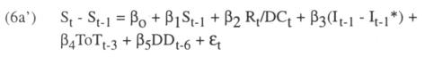
The first equation is similar to the one used by Svensson (1993) to test for mean reversion and interest rate differential. In this case, we are adding the reserve and domestic credit ratio, Rt/DCt to study the effects that the foreign reserves have on the exchange rate and on the lagged variables, terms of trade, ToTt-3 and domestic debt, DDt-6. These lagged variables reflect the fact suggested by Bosworth, Dornbush, and Laban (1994) that the changes in the terms of trade and domestic debt have a lagged effect on the exchange rate depreciation.
Where, St = nominal exchange rate composed of units of domestic currencies for one unit of foreign currency, It-1 = domestic interest rate, It-1* = foreign interest rate, Rt = foreign reserves, DCt = domestic credit, ToTt-3 = three months lagged terms of trade, DDt-6= six months lagged domestic debt6.
We should expect to have a negative relationship between the peso depreciation and exchange rate, reserve ratio, interest rate differential7 and terms of trade and a positive relationship with the domestic budget deficit, β1< 0, β2<O, β3<O, β4<0, and β5 > 0. If the exchange rate follows a mean reversion path, as is expected in a credible target zone system, the mean reversion implies that the higher the exchange rate, the lower the subsequent change in the exchange rate. A higher foreign reserve, with respect to domestic credit, will strengthen the exchange rate market with a large influx of foreign reserve in possible cases of higher foreign demand and speculative attacks. Increasing the domestic interest rate should decrease the peso depreciation8.
The second equation is derived from the central bank balance sheet. This model studies how the movements of reserves in the financial market and changes in the exchange rate can affect the interest rates differential.
Where, Rt = reserves, DCt = domestic credit, It = domestic interest rate, It* = foreign interest rate.
We should expect the interest rate differential to have a positive relationship with the exchange rate depreciation and a negative relationship with the reserve ratio, i.e Π1 > 0, and Π2 < 0. We should also expect that an increase in the depreciation of the exchange rate will increase the interest rate differential. If the domestic currency weakens, the demand for the currency will decrease, forcing the monetary authorities and commercial banks to increase the domestic interest rate to attract savings and avoid foreign market speculative attacks.
An increase in the foreign reserves will provide confidence to the investors for future exchange transactions, making the domestic currency more credible. Consequently, an increase in the reserve ratio may reduce the interest rate differential. In the case that the foreign reserve ratio gets closer to one (the foreign reserve magnitude is close to the domestic credit magnitude) the domestic interest rate will also become closer to the foreign interest rate, as the political risk as the only difference.
In the third equation, we analyze the effects that variables such as exchange rate changes, interest rate differential, terms of trade, and domestic and international debt have on the reserves. This model follows the Absorption approach, as we are interested in the difference between the reserve inflows and reserve outflows. We want to study what the main determinants are for the amounts of domestic savings (in foreign reserves) and foreign investments. We want to estimate the effect that the burden of terms of trade, domestic and international debt may have on the ratio of reserves and domestic credit.
Following López (1984), we are going to assume that reserves are a function of the exchange rate change, interest rate differential, terms of trade, domestic debt and international debt. Lopez presents a model assuming central bank intervention.
Where, Rt = reserves, DCt = domestic credit, ToTt = Terms of Trade, DDt = Domestic Debt, IDt = International Debt.
We expect the reserve ratio to have a negative relationship with exchange rate depreciation, a negative relationship with the interest rate differential, a positive relationship with the terms of trade, a negative relationship with the domestic debt and negative relationship with the foreign debt, i.e., Ω1 < 0, Ω2 < 0, Ω3 > 0, Ω4 < 0, Ω5 < 0.
If domestic currency is devalued, the demand for the foreign currency increases. If investors estimate that the monetary authority does not have sufficient foreign reserves to defend the domestic currency, they will accumulate the hard currency and capital flight will occur. The foreign reserve stock will be depleted and the reserve ratio will decrease.
We expect a negative relationship between the interest rate differential and the reserve ratio. Increasing the interest rate differential will make the domestic currency more attractive, and investors will move foreign reserves into the domestic currency market in order to take advantage of the greater returns. Increasing the domestic interest rate is a common policy which many developing countries use to make their domestic currency stronger with respect to a foreign currency. The terms of trade should have a positive significant relationship on the reserve ratio. The positive relationship indicates that as the exports increase proportionally more than imports, the economy will be getting more foreign reserves, increasing the reserve ratio.
The domestic debt should have a negative relationship with the reserve ratio. The domestic debt will be reflected in the debt that the government has accumulated in domestic currency. It will reflect the fiscal deficit and the amount of liabilities that the central bank has on its balance sheets. When the government borrows money from the public by issuing bonds, it will not affect the stock of domestic currency since no deposit is involved and consequently no money creation, but when the government is financed by the central bank, the domestic credit will increase.
The relationship between the international debt and the reserve ratio should be positive in the short run, but negative in the long-run. In the short-run, when private companies borrow foreign reserves, the new influx of foreign reserves will make the reserve ratio increase. If it is the central bank that borrows foreign reserves, the monetization of these loans will decrease the reserve ratio, but it will increase the stock of foreign reserves held by the public. On the other hand, in the long run, the private companies will need to obtain foreign currency to pay back the loans. In the case that the centra] bank has to pay its foreign debt, it can either use its own foreign reserves or it can create a sterilization policy to obtain funds from the investors to pay its debt. In any case, the stock of foreign reserve will diminish, lowering the reserve ratio.
We lump the three equations together as a set of variables to take into account information provided by all the equations on the system. So, the following three simultaneous equations are estimated:
Where St - St-1, It-1 - It-1*, and Rt/DCt are mutually dependent or endogenous variables, ToTt, DDt and IDt are exogenous variables, ToTt-3 DDt-6 are lagged variables and εt, ηt, and ωt are stochastic disturbance terms. Notice that although, It-1 may be controlled by the central bank, It-1* is not, and St - St-1 and Rt/DCt depend respectively on the demand of domestic and foreign currency. Using the order condition method we found that (6a) is just identified, (6b) is over identified, and (6c) is just identified.
4. Methodology
This paper uses different procedures to test the effects that different fundamental variables can have on the exchange rate. First, we test how several fundamental macro-variables imbedded in a system of equations affect each other and the exchange rate. In order to estimate these equations, we use instrumental variables such as two-stage least squares (2SLS), three-stage least squares (3SLS) and generalized method of moments (GMM). The instrumental variable technique is a general estimation procedure applicable to situations in which the independent variable is not independent of the disturbances. If appropriate instrumental variables can be found for the endogenous variables that appear as regressors in the simultaneous equation, the instrumental variable technique provides consistent estimates. Usually, exogenous variables and lagged exogenous variables in the system of simultaneous equations are considered best candidates since they are correlated with the endogenous variables through the interaction of the simultaneous system and are uncorrelated with the disturbances.
While 2SLS estimates the structural parameters on each equation separately, 3SLS estimates all the identified structural equation parameters together as a set. The major advantage of using the 3SLS technique is that, because it incorporates all the available information into their estimates, the estimates have smaller asymptotic variance-covariance matrix than single-equation estimators. The 3SLS estimator is consistent and in general is asymptotically more efficient than the 2SLS estimator. Since in a 3SLS procedure, if the system is mispecified, the estimates of all the structural parameters are affected, then we use 2SLS to compare both results. Given the likelihood of the existence of heteroskedasticity, GMM is used to compare with 2SLS and 3SLS results.
Second, we employ a general VAR approach to examine the dynamics of the relationship between the exchange rate depreciation, reserve ratio, and interest rate differential. We use the following VAR model:
Let the VAR(k) be:
![]()
Where,
y't = (St - St-1, Rt/DCt, It - It*), and β is 3x1 vector, Ω1, is a 3x3 parameter matrix,
εt is a 3x1 vector of the error terms, and t= 1,... Is the number of lags
St is the exchange rate, Rt is the reserve ratio, DCt is the domestic credit, It is the home interest rate, and It* is the foreign interest rate.
The Akaike information criterion is used to determine the initial lag length. Because estimated coefficients are not easily interpreted, we follow the common practice in VAR and look at the impulse response functions and variance decompositions of the system of equations to determine the implications of the relationships.
An impulse response function traces the response for several variables on shocks in the error terms of a given endogenous variable. The impulse response shows how an endogenous variable responds over time to a surprise (shock) change on itself or by another variable. If the error terms are uncorrelated, then these error terms depict the surprise movement in the corresponding left hand side endogenous variable.
The variance decomposition is used to measure the variance of the reaction of the endogenous variables. The forecast error of each variable at different time spans into the future and the changes from current to future changes can be obtained. The forecast error of the variance decomposition can suggest which other factors can have major influences on the behavior of a given variable.
5. Data
This paper uses monthly data from Chile for January 1979 to November 1997. The data used consists of foreign reserves, credit from the Central Bank, domestic reserves, imports, exports, claims on the government, GDP, foreign liabilities, domestic interest rate and foreign interest rate. Using the above variables, several composite variables are created such as the reserve ratio, terms of trade, domestic debt and international debt. The reserve ratio is given by the foreign reserve and domestic credit ratio. Terms of trade is the ratio of exports and imports, and the domestic debt and international debt are given by the claims on government and international liabilities as a share of GDP respectively. The lending rate was used for domestic interest rate and the U.S. Treasury Bill for the foreign interest rate. This data was taken mainly from the IFS CD-ROM. The GDP was taken from the Chilean Central Bank published on the Internet. The data used is converted to natural logs.
6. Statistics for Chile
The summary statistics for the different variables of Chile is presented in Table-1. The variables have been converted to logs, and the exchange rate follows the usual conversion of number of domestic units for one unit of foreign currency. We can observe that domestic reserves, claims on the government, and foreign liabilities have high volatility, and imports, exports, GDP, domestic interest rates have low volatility. The null hypothesis of skewness equal to zero is rejected on all the variables, except the domestic interest rate and foreign liabilities. It indicates that these variables appear not to have a symmetric shape. The null hypothesis of kurtosis equal to zero is rejected on all the variables, suggesting thicker tails on the variable distribution.
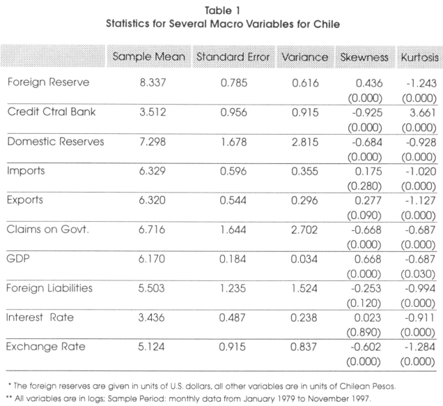
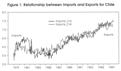
The means for the imports and exports are very similar values, 6.329 and 6.320 respectively.
7. Effects of Fundamentals over the Exchange Rate using instrumental Variables.
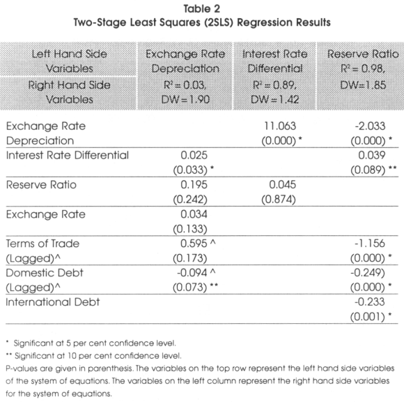
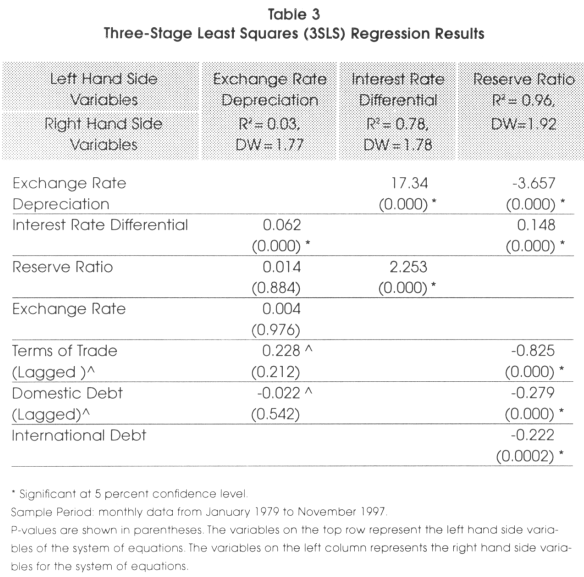
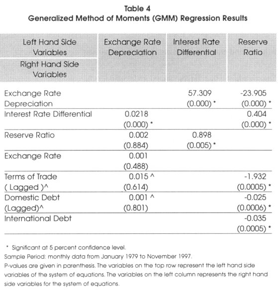
In this section we use Instrumental variables (IVs) to test the effects of several fundamental variables over the exchange rate. We estimate a two-stage least squares (2SLS), a three-stage least squares (3SLS), and a generalized method of moments (GMM) using the simultaneous equation introduced previously in this paper. We compare the three methods to find consistency in the results. Table 2, Table 3, and Table 4 show the results of the 2SLS, 3SLS, and GMM regressions respectively. In the 2SLS and 3SLS methods, the Durbin-Watson statistics show values close to two, suggesting no strong serial correlation. We find a low R2 for the first equation (i.e., exchange rate depreciation) in both methods.
Notice that when the R2 is high, say, in excess of 0.8, the estimated values of the endogenous variables are very close to their actual values, and thus the endogenous variables are less likely to be correlated with the stochastic disturbances in the original structural equations.
For the first equation from the system of equations, i.e..
We should expect β1 < 0, β2 < 0, β3< 0, β4 < 0, and β5 > 0. The 2SLS results shown in Table 2 do not support the relationship between the Chilean peso depreciation and reserve ratio, exchange rate, interest rates differential, domestic debt and the terms of trade.
The 3SLS and GMM results shown in Table 3 and Table 4 support the relationship between the peso depreciation, reserve ratio and exchange rate, but they do not support the relationship with the interest rate differential, the terms of trade and the domestic debt.
Both procedures give consistent results with respect to the interest rate differential and domestic debt. However, the only significant result is the interest rate differential. The mean reversion suggests that in the long run, the exchange rate has been stable. The reserve ratio relationship is not supported by the 2SLS, 3SLS and the GMM.
The most important finding is the relationship between interest rate differential and the peso depreciation. It is well known that monetary authorities use the domestic interest rate to control exchange rate depreciation and inflation. The idea is to make the domestic currency stronger by increasing the domestic interest rate. The target zone theory relies on the assumption that increasing the interest rate differential can reduce depreciation. However, our results show that the interest rate differential does not have the expected negative relationship with the peso depreciation (i.e., from Table 2, the coefficient found was 0.025, from Table 3, the coefficient found was 0.062, and from Table 4, the coefficient found was 0.021, all three results are statistically significant). This finding supports the idea that the Chilean interest rate may not have a strong influence on the peso. On the other hand, this positive relationship between interest rate differential and the peso supports the uncovered interest parity condition and second generation of target zone models, implying the Central Bank intervention was not credible9.
For the second equation from the system of equations, i.e.,
We should expect Π1 > 0, Π2 < 0. 2SLS, 3SLS and GMM results from Table 2, Table 3, and Table 4 in the third column of the three tables to show a positive relationship between the interest rate differential and the reserve ratio. While 2SLS produces non-significant results, 3SLS and GMM results are significant. The lack of effect of the reserve ratio in the value of the domestic interest rate can be accounted for by the higher volatility that the peso shows in Table 1. It also may indicate a higher degree of substitution between the peso and the U.S. dollar. That is, no matter how high the Chilean interest rate might be, investors and the public in general still prefer the U.S. dollar. The three methods, 2SLS, 3SLS and GMM show, as expected, a significant positive relationship between the interest rate differential and the peso depreciation.
For the third equation from the system of equations, i.e.,
We should expect Ω1 < 0, Ω2 < 0, Ω3 > 0, Ω4 < 0, and Ω5 < 0. 2SLS, 3SLS, and GMM presented in Table 2, Table 3, and Table 4 produce the same sign and significant values. The intersection between the four columns and the second row shows the expected significant negative relationship between the peso depreciation and the reserve ratio. On the other hand, if investors believe that the Central Bank has enough foreign reserves to counterattack any speculative attack, they will not speculate because their interventions cannot move the exchange rate out of the specified target bands.
We should expect a negative relationship between the interest rate differential and the reserve ratio. Increasing the interest rate differential should make the domestic currency more attractive and investors should move foreign reserves into the domestic currency market in order to take advantage of the greater returns. Increasing the domestic interest rate is a common policy in many developing countries to make their domestic currency stronger with respect to a foreign currency. However, the coefficients indicated in the fourth column and third row, shown in Table 2, Table 3, and Table 4, do not show the expected negative relationship. Again, as we previously found, the interest rate differential seems not to have any effect in strengthening the peso. This finding reveals that investors consider domestic currency a risky asset that requires a very high rate of return to make it attractive. The alternative of increasing domestic interest rates is inappropriate for many countries since it most likely would cause economic recession and fosters more poverty.
The terms of trade should have a positive significant relationship with the reserve ratio. This positive relationship indicates that as the exports increases proportionally more than imports, the economy will be getting more foreign reserves, increasing the reserve ratio. However, the values shown in the interception between the reserve ratio and terms of trade, shown in Table 2, Table 3, and Table 4, indicate a negative coefficient. This result can be explained by the statistics shown for the imports and exports in Table 1. Looking at the import and export means and variances in Table 1, we observe that their means are almost equivalent with low variances. The mean of the exports is 6,329 and the mean for the imports is 6,320. Figure 1 supports this argument since it shows a similar movement of both variables. These findings reveal that foreign reserves obtained by the exports could be used mainly to support the imports; consequently, the terms of trades did not contribute to raising the reserve ratio.
The domestic debt should have a negative relationship with the reserve ratio. The domestic debt is a reflection of the debt that the government has in domestic currency. It reflects the fiscal deficit and the amount of liabilities that the Central Bank has on its balance sheet. When the government borrows money from the public by issuing bonds, it does not affect the stock of domestic currency; however, when the Central Bank finances the government, the domestic credit increases. Since we are using the claims on government as a proxy to measure the government debt, an increase in the claims on government will either not affect the domestic credit or increase the domestic currency. In developing countries, taxes do not represent a strong source of income for the government; it usually is the Central Bank that finances the government. In this case, any increase of the domestic debt increases the domestic credit and consequently reduces the reserve ratio. This negative relationship is captured by the coefficients shown between the domestic debt and the reserve ratio in Table 2, Table 3, and Table 4.
Finally, the relationship between the international debt and the reserve ratio should be positive in the short run but negative in the long run. In the short-run, when private companies borrow foreign reserves, the new influx of foreign reserves makes the reserve ratio increase. If it is the central bank that borrows foreign reserves, the monetization of these loans increases the reserve ratio. In the long run, the private companies need to obtain foreign currency to pay back the loans. In the case that the central bank has to pay its foreign debt, it can either use its own foreign reserves or it can create a sterilization policy to obtain funds from the investors to pay its debt. In any case, the stock of foreign reserve diminishes, lowering the reserve ratio. The results shown in Table 2, Table 3, and Table 4 indicate the long-run negative relationship between the international debt and the reserve ratio.
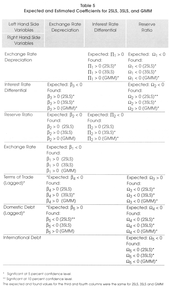
Table 5 shows a summary of the expected coefficients and the found coefficients after running the two-stage least squares, three-stage least squares and generalized method of moments regressions.
Same sign results were found for the second and third equations for procedures, 2SLS, 3SLS and GMM but not for the first equation of the three procedures. Table 6 presents a summary of the findings for the different relationships given by the 2SLS, 3SLS, and GMM procedures.
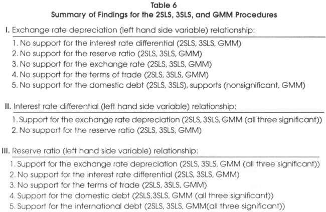
Figure 2 shows the relationship between the reserve ratio, domestic debt and foreign debt. Notice that the reserve ratio was higher from 1979 to 1983 but after 1983 the domestic debt and the foreign debt started to increase, supporting the negative relationship between the foreign reserves and the domestic and foreign debt.
Figure 3 shows the relationship between the reserve ratio and the terms of trade and the domestic debt. It shows that credit increases substantially more than terms of trade and reserve ratio after 1982. The growth of domestic credit was lower than foreign reserve between 1979 and 1982. Vertical axis is represented by domestic debt, terms of trade, and reserve ratio. The horizontal axis is represented by time.
8. Effects of the Fundamentals on the Exchange Rate using VAR
Since the impulse response functions and the variance decompositions are sensitive to the ordering of the variables in the VAR specifications, we use a Granger causality test to find the best single ordering that is correct. The usual procedure is to place the variables that may be more causal to the end of the ordering and those that are less causal at the front of the ordering. This is important since the first variable in the ordering dominates the impulse response and variance decomposition results. To establish the causal relationship between the exchange rate depreciation, reserve ratio and interest rate difference, we conduct a Granger causality test. The null hypothesis is that left hand side variables are not Granger-Caused by right hand side variables.
Table 7 shows the results for the Granger causality test. Since the p-values are not less than the level of significance of 0.05, we are not able to reject the null that left hand side variables are not Granger-Caused by right hand side variables with the only exception being the reserve ratio with interest rate differential as the dependent variable. According to these results, the least causal variable is the reserve ratio and the most causal is the exchange rate depreciation. The size of the impulse is a shock of one standard deviation above the mean of the residuals of the equation. The number of lags used was 10.
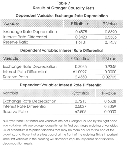
Figure 4 shows impulse responses of the interest rate differential and exchange rate depreciation when the reserve ratio is shocked. The impulse response shows how an endogenous variable responds over time to a surprise (shock) change on itself or by another variable. The size of the impulse is a shock of one standard deviation above the mean of the residuals on the VAR equation. The number of lags used is of 10. When the reserve ratio is shocked, the response on the peso depreciation is larger than the response on the interest rate differential. This figure shows that a negative shock in the reserve ratio produces a bigger negative effect on the peso depreciation and a positive shock in the reserve ratio causes a bigger positive effect on the peso depreciation.
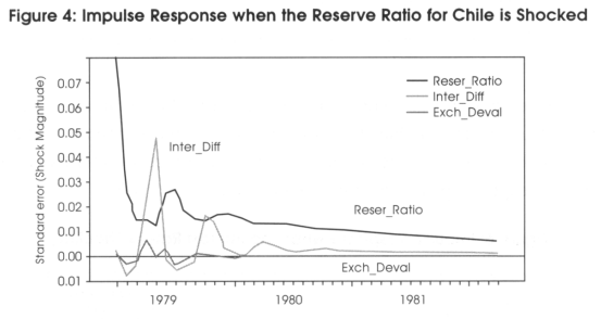
In general, a shock in the reserve ratio causes the peso to be more volatile than interest rate differential. The volatility produced either in the domestic credit or in the foreign reserve increases the volatility of the exchange rate.
Figure 5 shows impulse responses of the interest rate differential and reserve ratio when the exchange rate depreciation is shocked. The impulse response shows how an endogenous variable responds over time to a surprise (shock) change on itself or by another variable. The size of the impulse is a shock of one standard deviation above the mean of the residuals on the VAR equation. The number of lags used was 10.
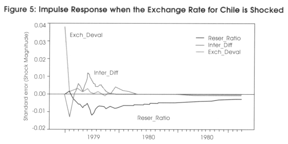
When the exchange rate depreciation is shocked (Figure 5), the interest rate differential responds sooner than the reserve ratio. At the beginning, the domestic interest increases; however, it decreases soon after. The reserve ratio has a negative response and keeps a negative trend for the duration of the shock.
When the interest rate differential is shocked (Figure 6), both the reserve ratio and the exchange rate have small reactions. The response of the peso change is almost zero, and the response of the reserve ratio is a small negative effect.
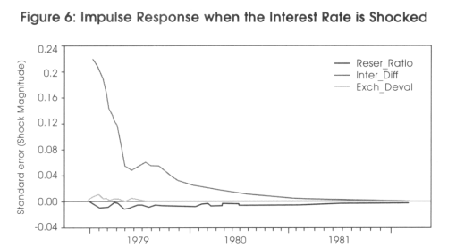
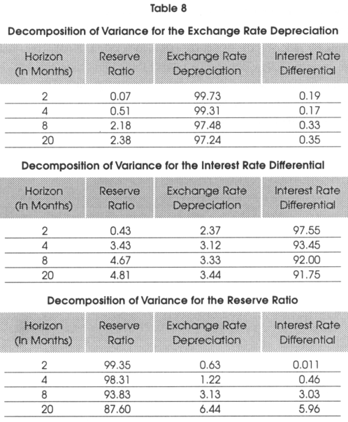
Table 8 shows the variance decomposition for the reserve ratio, exchange rate depreciation, and interest rate differential. The variance decomposition provides a fraction of the forecast error for each variable, we can attribute this to its own variance and to the variance of other variables. For example, Table 8 shows that the decomposition of variance for peso depreciation for a forecast horizon of 8 months is 2.18 per cent and is attributable to shocks on the reserve ratio and 0.33 per cent of the exchange rate depreciation is attributable to shocks on the interest rate differential. In general, Table 8 shows that the predominant external source of variation in exchange rate forecast error is from shocks on reserve ratio, the predominant external source of variation in reserve ratio forecast error is from shocks on the exchange rate and the predominant external source in interest rate differential forecast error is from shocks on the reserve ratio.
9. Conclusions
In this paper we examine the effects of foreign reserves and other fundamental variables on the exchange rate. We found that the interest differential does not have any effect on depreciation. This result does not support the target zone theory, which assumes a negative relationship between the exchange rate and interest rate differential, implying that the domestic interest rate can be used to manage the exchange rate. This is a very important finding since most international institutions and central banks use the domestic interest rate as a monetary tool to manage exchange rate, depreciation and inflation. We found that the foreign reserves support the exchange rate by reducing the exchange rate depreciation. Finally, the exchange rate and foreign reserves follow a negative relationship, supporting the assumption that increasing the foreign reserves appreciates the exchange rate. The levels of foreign reserves have not increased by favorable terms of trade but rather by foreign influx through debt and direct investment.
Notas
* School of Business, Le Tourneau University
Acknowledgement: We would like to thank Frank Lopez, Oscar Varela, and Gerald Whitney for helpful comments and suggestions. We also thank the participants at the 2000 FMA International meeting in Edinburgh, Scotland.
1 Edwards and Frankel (2002) provide the broad overview on this issue. Kaminsky and Reinhart (1998) compare the 1997 Asian and 1994 Latin America financial crises.
2 See for example, Svensson (1991). Lindberg, Soderlind, and Svensson (1993), Lindberg and Soderlind (1994), Werner (1995), Rangvid and Sorensen (1998), among others.
3 For example, the currency board system maintains a constant supply of domestic currency and changes the supply of foreign reserves accordingly. While a currency board system assumes that the fixed exchange rate can be maintained with sufficient foreign reserves, the target zone theory assumes that if the monetary authority intervention is credible, it will be able to maintain the exchange rate fixed around a central parity.
4 Sheen and Sheen (2002) show that the intervention by the central bank on foreign exchange markets is significantly influenced by interest rate differentials, profitability and foreign currency reserve.
5 A random walk with a drift term is given as: df = μdt + Φdz. Note that a drift would cause asymmetries in the analysis of the target zone model due to peso exchange rate depreciations.
6 In testing the number of logs to be used for ToT and DD, we ran an OLS regression using lags of 3 and 6 and found similar coefficient results for both lags. We decided to use a lag of 3 for ToT since exports and imports have been historically more responsive in the exchange rate than the domestic debt.
7 The negative relationship between exchange rate and interest rate differential is assumed by the target zone model. Some papers have also tested the interest rate parity condition, in this particular case the relationship should be positive which is the same assumption as the second generation of target zones.
8 With an increase in the interest rate differential, the interest rate parity condition assumes the spot exchange rate appreciates, the International Fisher theory assumes the predicted future spot rate depreciates, in both cases there is a positive relationship between exchange rate and interest rate differential. Whereas in the basic target zone model, an increase in the interest rate differential, appreciates the future predicted spot rate, suggesting a negative relationship between exchange rate and interest rate differentials or at least the exchange rate change would be smaller than the preceding period.
9 Since investors do not believe that the central bank intervention is credible, the predicted future spot exchange rate does not change (or might depreciate even more), and it becomes in an arbitrage condition.
REFERENCES
Bosworth, B., R. Dornbush, and R. Laban. 1994. "The Chilean Economy, Policy Lessons and Challenges". Brooking Institution, Washington, D.C.
Delgado, F. and B. Dumas. 1 993. "Monetary Contracting Between Central Banks and the Design of Sustainable Exchange Rates Zones". Journal of International Economics. 34, 201-224.
Flood, R. and R. Andrew. 1991. An Empirical Exploration of Exchange Rate Target Zones. Carnagie-Rochester Series on Public Policy, Fall, 35, 7-66
Edwards, S. and J. Frankel. 2002. Preventing Currency Crises in Emerging Markets. University of Chicago press.
Kaminsky, G. and C. Reinhart. 1998. "Financial Crises in Asia and Latin America: Then and Now". American Economic Review. 88, 44-448.
Krugman, P. 1991. "Target Zones and Exchange Rate Dynamics". Quarterly Journal of Economics. 669-682.
Krugman, P. and M. Miller. 1991. Speculative Attacks on Target Zones. Oxford: Oxford University Press.
Lewis, K. 1995. "Occasional Interventions to Target Rates". American Economic Review. 691-715.
Lindberg, H. and P. Soderlind. 1994. "Testing the Basic Target Zone Models on Swedish Data: 1982-1990". European Economic Review. 38, 1441-1469.
Lindberg, H., P. Soderlind, and L. Svensson. 1993. "Devaluation Expectations: The Swedish Krona 1985-92". Economic Journal. 103, 1170-1179.
Lopez, F. 1984. "The Effects of Various Credit Control in the Level of Internactional Reserves". Kredit and Kapital. January, vol 3. 404-416.
Rangvid, J. and C. Sorensen. 1998. "Determinants of the Implied Fundamentals from a Target Zone". Working Paper. Department of Finance. Copenhagen Business School. Denmark.
Sheen, K. and J. Sheen. 2002. "The Determinants of Foreign Exchange Intervention by Central Banks: Evidence from Australia". Journal of International Money and Finance. 21, 619-649.
Svensson, L. E. 1991. "Target Zones and Interest Rate Variability". Journal of International Economics. 31, 27-54.
— 1994. "How Long do Unilateral Target Zones Last?" Journal of International Economics. 36, 467-481.
Werner, A. M. 1995. "Exchange Rate Target Zones, Realignments and Interest Rate Differentials Theory and Evidence". Journal of International Economics. 39, 353-368.

