Electoral Systems and Corruption

 

 

Vincenzo Verardi^*, ECARES, CEPLAG

 

 

---

Summary

Recently, many scholars have tried to explain how electoral systems are linked to corruption. Several theories emerged but still no consensus has been reached. With a dataset of about 50 democratic countries considered over 10 years we try to understand which of the effects highlighted in the theoretical literature dominates. The results tend to show that larger voting districts (characterized by lower barriers to entry) are associated with less corruption, whereas closed lists tend to be associated with more. The latter effect is nevertheless not robust. In aggregate, we find that majoritarian systems tend to be associated to higher levels of corruption than proportional representations. An additional finding is that presidential regimes tend to be associated with more corruption than parliamentary ones.

---

Resumen

Últimamente, muchos estudiosos han tratado de explicar cómo los sistemas electorales se relacionan con la corrupción. Varias teorías surgieron, pero todavía no se ha logrado un consenso al respecto. En este estudio, con datos correspondientes a 50 países democráticos, considerados a lo largo de 10 años, intentamos comprender cuáles fueron los efectos dominantes más sobresalientes de acuerdo a la literatura teórica. Los resultados tienden a mostrar que los distritos electorales más grandes (caracterizados por menores barreras a la entrada) están asociados a una menor corrupción, mientras que las listas electorales pequeñas tienden a asociarse a mayores niveles de corrupción. Sin embargo, el último efecto no es robusto. En suma, encontramos que los sistemas mayoritarios tienden a estar asociados con mayores niveles de corrupción que las representaciones proporcionales. Adicionalmente encontramos que los regímenes presidencialistas tienden a estar asociados con mayores niveles de corrupción que en regímenes parlamentarios.

---

 

 

The aim of every political constitution is, or ought to be, first to obtain for rulers men who possess most wisdom to discern, and most virtue to pursue, the common good of the society; and in the next place,
to take the most effectual precautions for keeping them virtuous whilst they continue to hold their public trust.

James Madison (1751-1836)

1. Introduction

Corruption has always been present in the political life since the emergence of even primitive "political organizations". Temptations for power and wealth are strong especially when punishment is limited. To give an idea of how this problem has been part of politics for centuries, we cite Gaius Sallustius Crispus describing his own political experience. Gaius Sallustius Crispus was an historian and a politician born in 86 BC who forged his political career around 50 BC (the time of Julius Caesar)

Just like many other young men, my own first instinct was to commit myself completely to politics. Many obstacles confronted me. No one took any notice of self-control, integrity or virtue. Dishonest behavior, bribery. and a quick profit were everywhere. Although everything I saw going on was new to me - and I looked down on them with disdain - ambition led me astray and, having all the weakness of youth, could not resist. Regardless of my efforts to dissociate myself from the corruption that was everywhere, my own greed to get on meant that I was hated and slandered as much as my rivals.

G. Sallust Crispus, The Catiline Conspiracy I.5

From this quotation we immediately understand that temptations for abusing power are extremely strong (and have always been) for politicians and that without an appropriate system of monitoring and sanctions, the problem can worsen and lead, as happened for the fall of the roman Republic (McMullen, 1988), to an unsustainable situation.

This omnipresence of corruption is probably the explanation of why economists and non-economists have concentrated so much work on the study of its causes and its consequences. A natural question often asked is: Is corruption good or bad for development? The answer to this question is not trivial: there is a debate among economists on the topic. A strand in the corruption literature tries precisely to answer to this question and to understand the impact of corruption on efficiency and growth. Following the seminal work of Leff (1964), some economists have suggested that corruption might not necessarily be bad for growth, contrarily to what was thought previously, since it may improve efficiency. The idea is that, in a world with pre-existing distortions, corruption might allow for better efficiency. In other words, corruption can be seen as a lubricant in a rigid administration. Huntington (1968) even concludes that a rigid over-centralized honest bureaucracy is even worse than an over-centralized dishonest bureaucracy. Another argument that has been advanced to show the power of corruption in increasing efficiency is the fact that corruption can be seen as a selection process where only good firms survive (Beck and Maher, 1986; Lien, 1986). Indeed, if a political agent has the exclusivity in providing a necessary licence to only one firm among many, the political agent and the firms will start a bargaining process that will end with only the lowest-cost firm remaining in the game since it is the only one who can afford to pay the largest bribe. Francis Lui (1985), suggests that the efficiency enhacing power of corruption can also be seen through the minimization of waiting costs associated to queuing. With a very nice model, where the amount of the bribe to be paid is proportional to the opportunity cost associated to the time necessary to queue, he shows that the solution of the game is a Nash equilibrium with minimized waiting costs.

Even without adopting a moralistic view, we consider that these reasoning do not really match true life experience. In particular, these models almost all depart from the assumption that distortions are pre-determined which is not necessarily true since these distortions and corruption have a common origin.

At the opposite of these optimistic researchers, some others tend to show that corruption has a negative impact on the economy.

Myrdal (1968), for instance, suggests that when there are opportunities for corruption, instead of speeding up a process, politicians might try to slow it down in order to attract more bribes. This is clearly in opposition with Lui's (1985) results. This is probably due to the fact that Lui, in his model, supposes that both actors in the illegal transaction are "honest" and stick to a deal. If we remove this hypothesis of no moral-hazard and consider that someone else might come in the queue and propose a better offer to the public official, we believe that the model might give opposite results, in line with Myrdal's view, Boycko, Shleifer and Vishny (1995) criticize the validity of the optimistic models to describe real life experiences, since they rely on the hypothesis that corruption contracts are enforceable, which is clearly not always the case. These authors believe that these models are not robust to this change of hypothesis. To find a solution to this debate, many authors have concentrated their work on finding the relation between corruption and GDP growth to see who is right or which effect dominates. The main idea that emerged is that corruption has a negative impact on growth through its effect on investments (Bardhan, 1997). This result is confirmed by growing empirical literature (Mauro, 1995 or Wei, 1997). Thanks to these results, a consensus is emerging on the negative effect of corruption (even without any ethical considerations). A natural question at this point is, what should be done to reduce corruption?

Several potential solutions have been proposed in the literature. For example, one solution would be to increase public sanctions accompanied by high public wages or anti-corruption campaigns, but this is costly. Without minimizing the importance of these solutions, we leave them on the side here and concentrate, on the institutional factors that might play a role in the corruption reduction strategy.

Because of the intrinsic differences existing in the monitoring power of different institutions, there is no reason why corruption should be unrelated to electoral systems. If this is the case, and it is possible to identify which system is less prone to corruption, choosing the right system could be particularly interesting. Indeed, the effect of the adoption of an efficient system could be long-lasting and the cost would be limited since it is only associated with the fixed cost necessary to change the electoral law.

The first authors who have considered the role of electoral systems as a way of reducing corruption are Schumpeter (1950) and Riker (I 982). They are strongly against corruption and consider that one of the basic motivations for democracy is precisely the reduction of corruption, through electoral competition. They even affirm that the effect of electoral systems on corruption could be considered as a criterion for choosing one system instead of another.

The aim of this paper is thus to try to understand which systems are more prone to high levels of corruption and to give hints on which constitutional arrangement might be positive in the fight against it.

Before entering into the core of the research and explaining the theoretical predictions linking corruption and electoral systems, it is important to have a clear idea of what we define as corrupt behavior.

Corruption exists in different contexts and can mean many things. In economics, the most accepted definition of corruption is "the use of public office for private gains". It can be argued that this definition is very limited and that in real life, corruption exists outside the public sphere and can take different forms. Bardhan (1997) for instance, gives the example of a private seller that supplies a scarce good. Given that this good is not available for everyone or there are long queues to get it, people might be tempted to bribe the seller either to jump the queue or to have the opportunity to buy the good. He gives some examples like paying a higher price a "scalper" for a sold-out theatre play, tipping a "bouncer" to enter a night-club or using connections to find a job. This kind of corruption is important but is not our concern here. Another potential misunderstanding of the definition of corruption, is the confusion between corruption and illicit behaviour. Not everything that is illegal is corruption (such as for instance a murder or a robbery) and not all types of corruption are illegal (such as for instance some kind of political lobbying).

Bardhan (1997) makes an additional distinction. He emphasizes that there is a difference between "immoral" and "corrupt" transactions. For example paying a blackmailer in order to stop him from revealing some private information might be immoral but neither illegal nor corrupt. In this work we define corruption following the most accepted definition: corruption is the use of a public office for private gains. These gains can be monetary or of many other types. They can be for example patronage (the power of appointing people to governmental or political positions independently of their quality), nepotism (favoring relatives), job reservations, favor-for-favors or secret party funding.

In this paper, the goal is to test empirically the influence of institutions on corruption. Note that quantifying corruption is extremely difficult because of its secretness. We can say, without much doubt, that there is no objective measure of corruption available. The only way to quantify it is to use subjective measurements. Several indicators of corruption are available but only few are of a sufficient quality and can be used in a dynamic comparison of countries. The measurement we use here is the "International Country Risk Guide" (ICRG) indicator that we describe more in depth later. This indicator has the advantage of taking into account all these aspects of corruption at the same time.

As stated above, the aim of the paper is to test for the correlation between some constitutional features and corruption. Some papers have already been interested in this topic (Kunicova and Rose-Ackerman 2002, Kunicova 2000, Persson and Tabellini 2003) but all stay bounded to cross-sectional techniques remaining fragile to unobserved heterogeneity. In this paper we solve this problem by using panel data with a dynamic indicator of corruption. This also allows us to have more data points, thanks to the time dimension of our data. Given the information available, we can also make hard sample selections that allow us to work only with highly democratic countries remaining with sufficient degrees of freedom. This point is important since in non-democratic countries, electoral systems have very limited effects.

The structure of the paper is the following: after this introduction, in section 2, we present the theoretical predictions of the effects of the electoral system on corruption. In the third section we present the data we use and in the fourth our methodology. In the fifth we present our major findings and we conclude in the sixth.

 

2. Theory

Since Myerson (1993), only an extremely limited number of papers have analysed the systematic link existing between the electoral system and the level of corruption theoretically. Persson, Tabellini and Trebbi (2001) made an important step forward by summarizing the existing theories and by predicting additional effects. Looking at the existing theoretical literature linking electoral systems and corruption, about five hypothesis can be directly tested.

A first idea found in the literature, is that systems that promote the entry of many candidates and parties in the political decision sphere allow to keep corruption at a lower level than those who tend to favor the status-quo. The first formalization of this idea has to be attributed to Myerson (1993). In his paper, he considers a simple model in which votes allocate seats in legislature among parties having different levels of corruption. In this setting, the author assumes that there are only two policy alternatives "Left" and "Right". In the model, voters want to maximize their utility payoff represented by government policy minus their share of total costs of corruption for all parties. The assumptions of the model are such that, if all parties differ only in their corruption level, less corrupt parties will be chosen under all electoral rules. He considers the case where there are four parties L1, L2, R1, R2 where L means that the party is leftist and R rightist. The index 1 identifies well established corrupt parties while the index 2 identifies new coming "clean parties". With his model, he considers all the equilibria that exist under different types of electoral rules. He gets to the conclusion that in systems where the barriers to entry are high (that is to say when the district magnitude is low) corruption will tend to be high since a well established party will be hard to remove from office at a low ideological cost. Voters will prefer to vote for the already present corrupt party, that has an ideology he likes, instead of voting for the new non corrupt party (with the same ideology), since this could give the victory to the opposite ideology party if no other voters deviate from the status-quo equilibrium. To test if his model is confirmed by real world data, we can check the following hypothesis:

H1. Countries with larger mean district magnitude have less corruption

A second feature that has been identified in the literature, is the role of the electoral formula and in particular the existence of closed lists in promoting corruption. When voters can choose for the candidate they prefer, there is a direct link between the candidate and the voter. If the politician does not behave properly and, for example accepts bribes, he knows that he will most probably be removed from office (from electors) in next elections, given that he is tightly monitored by them. This encourages him to behave properly. At the opposite, when candidates are elected under the cover of closed lists, the probability of being elected is not a function of their behavior but of their position in the list. Since their position on the list is not necessary dependent on their quality but on the preferences of the leader of the party, the constraint to behave properly is very limited. A nice "Holmstrom (1982) style" career concern model for this can be found in Persson and Tabellini (2000). The hypothesis to test in practice would be of the type:

H2. Countries using closed lists, for the election of representatives, have more corruption

A third point, that can be seen as a combination of the first two is that if the barriers to entry effect dominates the closed list effect, majoritarian systems will be more corrupt than proportional representations. To test for this in practice, we will have to see if:

H3. Majoritarian systems have less corruption that proportional representations

A fourth point is on the regime type and not on the electoral rule. The idea in the literature is that, if there are not enough checks and balances, the president can centralize legislative, agenda-setting and veto powers (Kunikova and Rose-Ackerman, 2002) and behave as an "elected autocrat" which could be a cause for the abuse of power. Following the definition of presidentialism of Persson and Tabellini (1999)¹, that we use in this work, we think that this effect should not play any role. Indeed, we consider as a presidential regime, a system where the separation of powers between the president and the legislative organ should protect against the abuse of power of each organ, so we do not think that this effect plays heavily. We could even imagine that this separation of powers might force better behavior. Nevertheless, a president can stay in office only a limited number of years. Often he cannot even be elected more than once. This impossibility of being re-elected gives him no advantages in behaving properly. On the contrary in parliamentary regimes, the government can stay in office as long as it has the support of the people. We think that this effect should be the reason why presidential regimes might be associated to higher levels of corruption than parliamentary ones. The hypothesis to test is then:

H4. Presidential regimes have higher levels of corruption than parliamentary regimes.

It can be argued that it is well known that presidential and majoritarian systems have most probably smaller governments than parliamentary regimes and proportional representations. Indeed, in these systems, Persson and Tabellini (2000) and Milesi-Ferretti et al. (2001) have shown (under some conditions) that the size of government will be small since politicians tend to orient public expenditures towards what is preferred by powerful minorities instead of broad coalitions of voters. This under-provision of certain types of expenditures can be seen as an opportunity for public officials to propose them illegally. Corruption could then be higher because it would be a substitute to public expenditures not delivered legally and could be indirectly linked to electoral systems.

The final hypothesis we want to test is precisely this indirect effect of majoritarian and presidential systems on corruption through the under-provision of public goods. The hypothesis to test in practice, is of the type:

H5. In majoritarian and presidential regimes, the size of the government is small and there will be an under-provision of public goods. To provide the public good needed anyway, some public officials will accept bribes. Corruption will be higher under presidentialism and majoritarianism than under proportional representations and parliamentary regimes.

Except for hypothesis H3 that is highly correlated with hypotheses 1 and 2, all the others have to be tested simultaneously to avoid problems of omitted variables biases. The strategy will thus be the following. We first test hypotheses 1 and 2 together with hypothesis 5. Then in a second regression, we test hypotheses 4 and 5 together. H5 will be considered in the robustness section since it is an hypothesis of quality of the specification of Hypotheses 1 to 4.

 

3. The Data

As explained briefly in the introduction, in this paper we use some panel data methods. These methods have several advantages over standard cross-sectional or time series estimators. The first big advantage is that the number of data points is much larger. In our case this is particularly important. Indeed, in several studies on corruption, the analysis was performed on a very limited number of cross-sections (countries). Since the number of countries in the World is limited, it is impossible to run a cross-country analysis keeping the number of degrees of freedom high. Using panel data allows thus to increase efficiency and to reduce the problems of collinearity. In our case, the additional availability of data is even more important than that. Indeed, electoral systems do not mean anything in autocracies where elections are either non-existent or non relevant. To understand effectively the relationship between electoral systems and corruption, we should work only with sufficiently democratic countries. In the beginning of the nineties there were only about 50 countries that could be considered as sufficiently democratic and that could be used for this analysis. The result is that, if we want to test for the correlation between electoral systems and corruption, we should either insert in our dataset also non-democratic countries (which is difficult to justify) or to work with panels. Otherwise, the degrees of freedom will be too low to infer anything.

When we analyze previous studies we see that, among the 82 countries they consider, Persson and Tabellini (2001) keep 23 countries that cannot even be considered as lowly democratic² and 33 countries that cannot be considered as highly democratic³ otherwise, using their 20 explanatory variables, they would have extremely low degrees of freedom. In Kunicova and Rose-Ackerman (2002) or Kunicova (2000), we find similar problems.

In this paper we try to use the best available data but also the most suited methodology. In the next section, we explain in detail how we believe corruption data should be used and which specification should be adopted for the empirical analysis.

3.1 Corruption

As we have specified many times previously, we want to work with a panel dataset. For this, we need an index of corruption that changes over countries and over time. Not many dynamic indicators of corruption are available. As far as we know, there are only two that are of sufficiently high quality. The first is the famous Transparency International Indicator that has been calculated for several years on the basis of a set of other indicators. This is of a high quality and has been available for 5 or 6 years. However, we prefer not to use it because it is based on heterogenous calculations that are not comparable across time. This could cause severe biases. Instead, we use the "International Country Risk Guide" (ICRG) measurement of corruption. The ICRG is a publication of the Political Risk Service (PRS) group that provides financial, political and economic risk ratings for 140 countries. Since 1980, the ICRG has been evaluating both the significant developments and subtle factors concerning corruption in 140 countries. One of its strengths is that it manages to identify major changes even when popular opinion points in different directions⁴

The corruption measurement is an assessment of corruption within the political system. It considers both financial corruption (demands for special payments and bribes for services) and excessive patronage, nepotism, job reservations, 'favor-for-favors', secret party funding, and suspiciously close ties between politics and business. It lies between a lower bound (0) that means total corruption at all levels and a higher bound (6) that means no corruption at all. For simplicity we recode it the other way round form 0 to 6 (with 0 meaning no corruption and 6 total corruption). The scale is ordinal but the distance between the levels remains constant.⁵ To calculate this, the ICRG staff collects political information data, and converts it into points. To ensure consistency, both between countries and over time, points are assigned on the basis of a series of pre-set questions and checked by ICRG editors that round the index to the closest entire number. The set of questions used depends in turn on the type of governance applicable to the country in question. Given how data are constructed, we understand that the only available information is not the true value of the corruption measurement but its closest integer. For instance, if we have a true level of corruption of 3.26/6 in a country and a true level of corruption of 2.74/6 in another, it will be coded in both cases as 3/6. Even worse, if a country sees its true level of corruption changing from 3.49/6 to 3.51/6, even if corruption did not change much, the indicator would say that we jumped from 3 to 4. The results of the linear regression are thus not really appropriate but will be presented anyway for comparisons and to have an idea of the size of effect. We will thus not consider the ranking as linear and use the adequate techniques.

To give an idea of our data, we present here below, in table 1, some descriptive statistics on our corruption index.

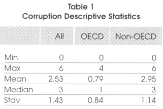
From these simple statistics, we see that corruption is much more concentrated (around a lower mean) in OECD countries than in non OECD countries. Among these countries, the lowest values can be found in countries like Canada, Denmark. Finland, Iceland, Luxembourg, the Netherlands, New Zealand, Norway, Sweden or Switzerland while the highest values can be found in Turkey (especially in the late eighties, early nineties), Greece and Italy. In the non-OECD countries, the highest levels of corruption can be found mainly in sub-Saharan Africa and Latin America.

3.2 Political Data

In this study we mainly use three political indicators to test the hypothesis formulated in the introduction.

a) The first, is a variable concerning (the In of) the district magnitude (lmdmh). This measure, is an indicator of the average number of representatives elected in each district. It goes from 1 in perfectly plurality single member districts systems up to 150⁶. The maximum is reached in pure proportional representations⁷ where the unique district is the entire country. The formula is:

This variable is taken from the "Database on Political Institutions" (DPI) This dataset contains 113 variables for 177 countries from 1975 to 1995 and was compiled recently, by the Research Group of the World Bank (Beck et al (1999)).

b)  The second is a dichotomic (cl) variable that takes the value 1 if at least part of the parliament is elected under a closed list system and zero otherwise. This variable comes from the DPI as well. About 66 percent of the countries in the dataset have, at least for part of the parliament, members elected under a closed list. This proportion does not change even if we consider only highly democratic countries.

c)  The third variable (ma) is a variable coded equal to one if the system is majoritarian and zero otherwise. Given that in the World many countries are neither pure majoritarian nor pure proportional systems, to code a variable equal to one, we check if either the system is a pure majoritarian or if the majority of the assembly is elected under the majority rule.

d)  The fourth political variable we analyse here (pres) is a dummy variable that takes the value 1 if the system is presidential and zero otherwise. Following Persson and Tabellini (1999), to code our presidential dummy variable as equal to one (presidential), we simultaneously check the degree of authority of a popularly elected president over the cabinet and the extent to which the survival of the executive and assembly powers are separate. Under such rules, a country can have an elected president and can be classified as parliamentary. A typical example of this is France where the government, holding proposal powers over economic policy, is dependent on the legislature and thus is coded as parliamentary. In the total sample there are 55 percent of presidential regimes and 45 percent of parliamentary regimes. If we make the same sample selection as above and consider only the highly democratic countries, we see that there are 35 percent of presidential regimes and 65 percent of parliamentary regimes.

3.3 Control variables

Besides the time dummies that are considered in all the specifications to take into account common shocks for a given year and influencing all the countries, the control variables in the regressions are of two types. A first type, regroups all the variables that are time varying and that have been suggested by the literature as influencing corruption. A second type are time invariant variables, that have also been considered in the literature and that have to be considered when we run an error component specification to avoid inconsistency due to omitted variables.

The variables of the first type are:

a)  The logarithm of GDP (lgdp) to control for the level of economic development, as suggested by Persson and Tabellini (2001).

b)  The logarithm of the population (lpop) considered by Persson and Tabellini (2001), to control for the size of the country.

c)  The degree of openness (open) of the market (measured as the sum of exports and imports in percentage of GDP) as used by Ades and Di Telia (1999) to control for the high correlation between openness and corruption.

d)  The level of education (educ) measured as the average number of secondary school attained in the population older than 24 years (as considered by Persson and Tabellini, 2001)

e)  The number of years the party of the chief executive has been in office (yrsoffc) to control for the effect predicted by Geddes (1997)⁸ stating that "when a new party comes to power, it will have greater incentives to reform corrupt practices of its predecessors"

f)  The level of democracy (democ) considered by Fisman and Gatti (1999).

The first three control variables come from the IMF yearbooks, the level of education comes from Barro and Lee (2000), the number of years the party of the chief executive has been in office comes from the DPI (Beck et al, 1999) and the level of Democracy comes from the Polity III database (Jaggers and Gurr, 1995)

The variables of the second type are:

a) Regional and geographic dummies. These are dichotomic variables that identify 8 regions of the world, namely: East Asia and Pacific (reg_eap), Eastern Europe and Central Asia (reg_eca), Middle East and North Africa (reg_mena), Southern Asia (reg_sa), Western Europe (reg_we), North America (reg_na), sub-Saharan Africa (reg_ssa) and Latin America (reg_lac)⁹, if a country is landlocked or not (landlock), if the country exports primary products other than oil (non-oil) or if the country exports mainly oil (oil).

b)  Legal origin dummies. As suggested by La Porta et al. (1999) and Treisman (2000) these should influence corruption. We identify three: British (leg_british), French (leg_french) and Socialist (leg_socialist) legal origin

c)  Ethnic and cultural variables such as the Ethno-linguistic fractionalization (ethfrac) that has been suggested to be correlated to corruption by La Porta et al. (1999) and a dummy identifying if the country is catholic or not (catholic).

d)  The degree of federalism (fed), coded from 1 to 3 (with 3 meaning highly decentralized) as suggested by Fisman and Gatti (1999).¹⁰

 

4. Methodology

In this section we briefly describe the methodology used for the estimations. An important feature of our estimations is that we want to see the impact of political, time-invariant variables on a time varying variable. A pooled regression with a common constant is not interesting in our framework because of the presence of unobserved heterogeneity, so, we have to use an error-component specification. The country fixed-effect estimation would be a natural choice if we had only the time-variant variables. In our situation, it is not the case and, because we have also time-invariant variables, there would be a problem of perfect collinearity between the country fixed effects and these time-invariant variables. This would make the estimation impossible to run. On the contrary, a regional fixed effect with an error component effect specification, to control for differences existing between countries in a same region, is perfectly suited for this, but cannot be used without considering many problems that can exist and that we describe in the next sub-section.

4.1 Specification

Suppose that we have to estimate an equation of type:

It is commonly accepted that all factors that affect the variable y_it but have not been included as regressors, can be summarized by a random term. This leads to the assumption that the u_i are random. In our framework, there is no justification for treating the individual effects as uncorrelated with the other regressors and considering u_i as random, given that there are major differences between countries that cannot be considered naturally as random. Following Greene (2000), we can say that using an error component model, in our case, may suffer from inconsistency due to omitted variables. What we should do then, before using this specification, is to control for variables (that do not change over time) that have been suggested in the literature as influencing corruption. If we control properly, what will remain in the error could then be considered as random. How will it be possible to understand if we controlled properly and that we do not have omitted variables? A natural idea is to run a Hausman test and check if the regional fixed-effect error component estimator and the country effect estimator do not differ systematically. If the tests does not reject the null hypothesis of no systematic difference between the estimates, we will then conclude that the non-stochastic heterogeneity of ui has been removed and what remains is random.

4.2 Error Component Interval Regression

The structural interval regression model for a possibly unbalanced panel of data would be written¹¹:

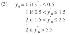
The problem here is that y^*_it is not observed. We only observe y_it that takes different values depending on the value of the latent variable. If the true value of the corruption indicator is lower than 0.5, our indicator will be given a zero value. If the true value lies between 0.5 and 1.5, our indicator will be coded as equal to one, and so on. Note that the distance between two levels of the indicator are always a unit. The difference with an ordered logit where the only information available is the ranking of alternatives is huge since here a difference in magnitude is available. In other words¹²,

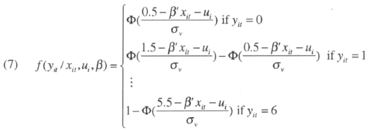
if ε_it is considered as standard normal the panel nature of the data is irrelevant. Therefore¹³:

If we make an error component assumption, and assume that:

we make the usual assumption that u_i, and v_it are i.i.d. normally distributed, independent of, X_i1,...X_it, with zero means and variances σ² _μ and σ²_v ;. ε_it ~ N(σ²_μ + σ²_v).

Using f as a generic notation for density or probability mass function, the likelihood function can be written as:

For the random effect interval regression model, the expressions in the likelihood function are given by:

The density of u_i is:

The joint probability is then:

The integral (9) must be computed numerically through the algorithm described in Butler and Moffitt (1982). Basically, the idea is that the function is of the form:

which is amenable to Gauss-Hermite quadrature for computation. The resulting coefficients are the Error Component Interval Regression estimators.

4.3 Summary of the Procedure

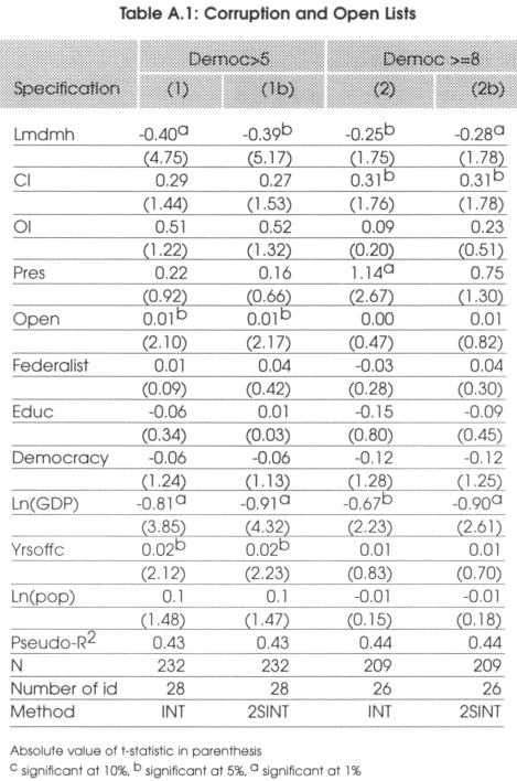
For the sake of clarity, we summarize here briefly the procedure explained above. The procedure is in two steps: the first step consists in running a country fixed effect interval regression model.¹⁴ Then we run a error component regional fixed effect interval regression model and run a Hausman test and check if the results of these two estimations differ systematically. If we see that this is not the case, the error component regional fixed effect can be considered as appropriate and the results can be analyzed.

 

5. Empirical Results

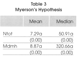
Before presenting the empirical results and testing the effects presented by the authors, it is important to check if the basic hypothesis of the model of Myerson (1993) are respected, that is to say if in proportional systems, barriers to entry are lower (and the number of parties higher) and if the mean district magnitude in majoritarian systems is low and close to 1. The descriptive statistics we show are associated to the sub-sample of countries having a level of democracy superior to 5 out of 10 for the reasons explained previously. Ntot is the effective number of parties measured as (1/HFI) where the denominator if the Herfindahl fractionalization index and mdmh is the average district magnitude in the lower house.

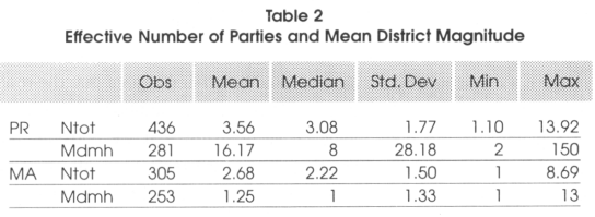
From the descriptive statistics presented in Table 2 above, we see that indeed the effective number of parties is on average higher in proportional representations (3.56) than in majontanan systems (2.56). We also see that the mean district magnitude is on average 1.25 in majoritarian systems and 16.17 in proportional representations.¹⁵ The median average district magnitude is also much higher in proportional representations than in majoritarian systems. The hypothesis of Myerson's model seem thus to be perfectly in line with the reality. Are these differences statistically significant? To test for this, we run a two-sample t test of the hypothesis that Ntot and mdmh have the same mean within the two groups, majoritarian and proportional representations (the two-sample data are not to be assumed to have equal variances). To check if the median is the same in the two groups, we run a nonparametnc x² 2-sample rank-sum test on the equality of medians. The results are reported in Table 3 and strongly support our precedent findings. For the comparison of means test we show the t-statistic associated to the test with the p-value associated to it in parentheses below. For the equality of medians test, we show the x² associated to the test with the p-value associated to it below.

After this brief statistical introduction needed to show that the hypothesis of Myerson are empirically founded, we present our major findings. If the hypothesis of Myerson were not confirmed by the data, it could have been argued that the model was not suited to check for real life results. In 4 and 5, in addition to the estimation technique explained in the methodological section and that we consider the most appropriate (defined INT in the methodology row in the tables), we also give, to allow comparisons, the result of the same estimation but using a linear Error Component Regional Fixed Effect regression (called ECRFE). Finally, to take into account the possible endogeneity of GDP with respect to corruption, we also give the result of the interval regression where GDP has been instrumentalized by five years lagged GDP (called 2S1NT). In Table 4 we present the result of the Hausman test of appropriateness of the error component specification. We see that in all the cases the error component specification is appropriate. In our estimations, we divide our sample in two sub-samples. In the first, that we call broad, we consider all the countries and all the years in which the level of democracy is higher than 5 out of 10. In the second that we define narrow, we consider all the countries and years in which the level of democracy is higher than 8 out of 10.

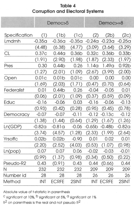
To remain coherent with the theoretical section, we give the result of each test of hypothesis defined separately. For the first hypothesis tested, in the light of the results presented in Table 4, we see that countries with larger mean district magnitude can be considered as having less corruption. We can conclude that this hypothesis cannot be rejected. Indeed, when we consider both the large sample and the narrow sample, we see that the coefficient associated to the district magnitude is negative and highly significant be this in specification 1 (and 1c) and 2 (and 2c).

For the second hypothesis, that is to say that in countries where some of the representatives are elected under a closed list, corruption should be higher, we find evidence that this seems to be true. Indeed in both specification 1 and 2, we see that the coefficient associated to this variable is positive and significantly different from 0. Given that there is probably some collinearity between the district magnitude and the fact of having a closed list, it is probable that the standard errors are inflated and that this coefficient is even more significant.

We see that hypothesis 4 has to be rejected by our data. Indeed, from Table 5, ma has a positive and significant coefficient. This means that it is significantly different and superior to proportional representation. This also means that the access to entry effect apparently dominates the monitoring effect of hypotheses 2 and 3.

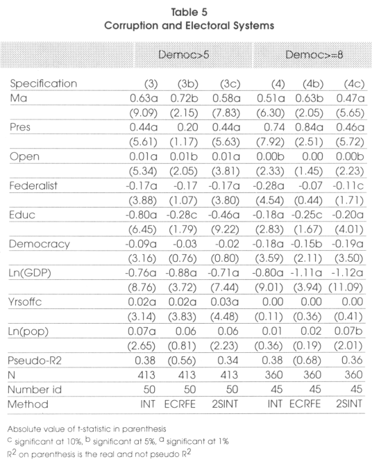
As far as the fourth hypothesis is concerned, we see that in lowly democratic countries, the presidential dummy doesn't seem to be significant while in highly democratic countries, presidential regimes seem to be more corrupt than parliamentary ones. This tells us that we cannot conclude anything about the correlation between presidentialism and corruption in lowly democratic countries but, as explained, in low-level democratic countries, the effect of electoral systems in reducing corruption is extremely limited.

As far as the size of effect is concerned, it would have been probably better to consider marginal effects given that we are in the context of non-linear regressions. Nevertheless, we believe that OLS can be considered as a sufficient approximation to have an idea of the magnitude of the difference between systems. As far as the district magnitude is concerned, when the average district magnitude increases by 100 percent the corruption index would decrease by 0.25 units. As far as closed lists are concerned, we can say that if a country changes from a closed list proportional system to an open list or personal vote one, corruption would decrease by 0.33 units.

Note that the pseudo-R² calculated is the one proposed by Amemiya (see Verbeek, 2000):

Where log L₁ denote the maximum likelihood value of the model of interest and log L₀ denote the maximum value of the likelihood function when all parameters, except the intercept, are zero. N is the total number of observations. Given the size of the sample, The Mc-Fadden R² gives similar results.

In Table 5, we see that changing from a majoritarian system to a proportional representation would reduce corruption by 0.63 units while abandoning a presidential system in favor of a parliamentary one, would reduce corruption by approximately 0.84 units. As far as the effects on other variables is concerned, even if we are not really interested in it, we see that, except for openness where the results might be questionable, all the results seem to go in the expected direction. Indeed education, development and democracy are negatively correlated to corruption while the number of years in office of the chief of the executive is positively correlated to it. In the literature the case of Italy is often cited since to reduce its corruption, Italy has made some constitutional arrangements. It changed from a pure proportional representation to a mostly majoritarian system. Indeed 475 (75 percent) of the elected representatives are now elected in single member districts while for the remaining 25 percent (155) the system is proportional representation with closed party-list on the basis of national voting results Myerson (1993) thinks that this is a step in the wrong direction since now the barriers to entry for new candidates will be higher and changes will be more difficult to achieve. Persson and Tabellini (2001) think the opposite given that they say that the number of elected representatives under party lists will diminish with the reform and the career concern effect will be strong. Indeed, for them, politicians will behave better now since their success in the next elections will be more conditional on their behavior than on the preferences of the chief of the party. What we find is that the effect of lists is less important than the effect of barriers to entry. Except in the case of already low district magnitude proportional representations, going towards a single-member district legislation should increase corruption. In all the models specified above, we must be sure that the model is applicable. For this reason we present in Table 6 the results associated to the Hausman test (as described previously) that support the fact that our methodology is well suited here.

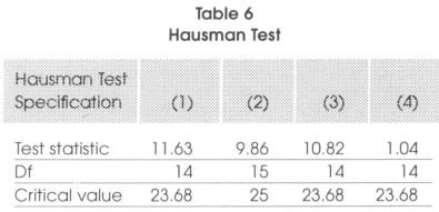
We see that in all our specifications the test statistic is inferior to the critical value of the x_df² The hypothesis that there is no systematic difference between the country fixed effect and the error component regional fixed effect specification cannot be rejected.

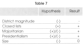
For the sake of clarity, we present a table where we summarize the predicted effects, as well as the empirical findings over the implications of some of the features of electoral systems on corruption.

 

6. Sensitivity Analysis

To test the robustness of the results, we add additional control variables which are usually used in the literature, and run our basic regression (1) plus these control variables and check if the coefficients associated to the explanatory variables we are interested in remain consistent with our previous results. The methodology adopted is the one proposed by Sala-i-Martin (1997) and described in the appendix. Keeping the same notations as before, the objective is to test for the robustness of coefficients associated to the electoral systems dummies. The methodology suggests to estimate an equation of the type:

where W_it is a subset of variables taken from a pool of variables that have been considered as influent in explaining corruption in previous studies and h is the coefficient associated with it. The extreme bound analysis consists in varying the subset Wit included in the regression and to consider the widest range on the variable of interest for which hypothesis testing does not reject the null. In other words, we run all regressions including all the combinations of one, two and three variables included in W_it as control variables, and we then check whether the coefficients associated with the electoral system remain stable.

The additional control variables considered for this sensitivity analysis are the degree of influence of religion on politics (REL), an index of the degree of external conflict risk (EXTCONF), the degree of influence of military in politics (MILIT), an index of the degree of openness of the recruitment of the executive (OPENEXEC) and the index of political cohesion in the parliament (IPCOH). Given that we are only interested in the effect of electoral systems that play fully only in highly democratic countries, we will only make a robustness check on the narrow sample and after having corrected the GDP for endogeneity. This procedure gives a total of 25 regressions for each methodology, that is 50 (extremely computer intensive) regressions for the two specifications. Given that there are no missing data for any additional variable considered in the robustness check, the number of observations is 209 for 26 in the first specification (Imdmh vs cl) and 362 for 45 countries in the second specifications (ma vs mixed). The results of the analysis are summarized in table 8.

From the results we see that for CL (that is non-normal) the robustness technique tends to confirm that they are not robust. On the contrary, it turns out that PRES can be considered robust at 99.94 percent which is extremely high. In conclusion, we can say that the lmdmh, MA and PRES are strongly robust, while CL is fragile.

Now that we have seen that there seems to be a link between electoral systems and corruption, it might be argued that the only thing we capture is the fact that these systems are associated to different sizes of government which could mean that in smaller governments¹⁶ there might be an under-provision of public goods and this could explain why different systems are associated to different levels of corruption. It is thus important to test for hypothesis 5 (that is to say that corruption cannot be considered as a compensation for a lower provision of public goods due to the electoral system). To do so, we run three regressions: in the first, we do not consider the electoral system dummies and just control if the size of the government has an effect on corruption. If it has no effect on corruption, then we will say that hypothesis 5 has to be rejected. Instead, if it has an effect, we run a second regression that is the same as the one in the previous stage but where we add the electoral system variables. Now if the SIZE (measured as the ratio total expenditures in percentage of GDP) variable becomes non significant and the system dummies remain significant, this means that the only effect the size of the government has on corruption is through the electoral systems and thus, we reject hypothesis 5 (because the indirect effect is insignificant). If both are significant the effect is both direct and indirect while if only the SIZE is significant it means that the only effect that is significant is the indirect effect and the direct one is inexistent. In Table 9 here under, we present the findings associated to the variables of interest but, for the sake of clarity, we do not report the results associated to the control variables We only make this analysis on the majoritanan and presidential dummies since the district magnitude and the existence of closed lists were characteristic that are already considered in the previous subdivision.

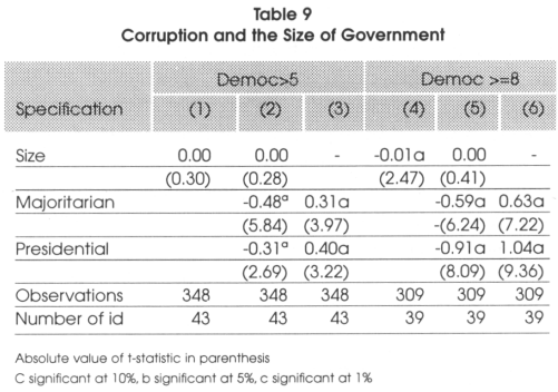
From the results here above, we see that in the broad sample, the size of government has no effect on corruption so, the indirect effect that could exist because of the under-provision of public goods has to be rejected. In highly democratic countries, we see that the effect of the size of government tends to influence corruption, but, we understand from model 5 in Table 9 that this just because there is a correlation between SIZE and electoral systems. Once we correct for this, the effect disappears. The effect of electoral systems found previously seem to be direct through the monitoring power of electoral systems and not through its effect on the size of government.

 

7. Conclusion

In this paper we used high quality data to test for the correlation between electoral systems and corruption. Using what we believe to be the most appropriate methodology, we find that the relations between constitutional features and corruption are multiple. First we find that when the district magnitude increases, that is to say when the average number of representatives elected in each district rises, corruption decreases. This is related to the hypothesis of lower barriers to entry proposed by Myerson (1993). Second we found that in countries where some of the representatives are elected under the cover of closed lists, corruption tends to be higher. This is related to the career concern hypothesis proposed by Persson and Tabellini (2001). Nevertheless this result is somehow fragile and seems to be related to the model specification.

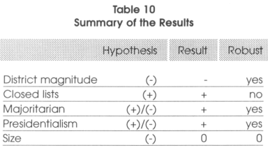
Given that low district magnitudes is typical of majoritarian systems we find that these systems are more corrupt than proportional representation and that the high district magnitude effect dominates the fragile closed-list effect. Majoritarian systems thus tend to be more corrupt than proportional representations. In addition, we deduce that the effect of electoral systems is direct and does not go through an eventual under-provision of public goods. Finally we found that presidential systems tend to be more corrupt than parliamentarians. We can summarize the results in a simple table. In the first column we present the name of the variable of interest, in the second its expected effect on corruption and in the last two columns, the sign of the effect obtained in the regressions¹⁷ and if the result is robust.

We could conclude that for corrupt majoritarian or presidential systems, a potential solution to reduce corruption might be to abandon the actual system and adopt in the first case an open list proportional representation and in the second a parliamentary regime. In terms of countries, our interpretation is, if the only objective is the reduction of corruption, for India, Bangladesh or Chile it would be a good idea to move towards a proportional representation system and for Latin American countries in general, it might be a good idea to move towards parliamentarism.¹⁸ In the case of closed-list proportional representations, given that we have seen that open lists are less negative for corruption than closed lists, maybe a solution would be to let the people vote for a list where it is possible to change the order of the candidates. In such a way the barrier to entry would be limited and the career concern argument would still hold. We could again take the case of Latin America as an example. Indeed in that region, almost all the systems are proportional representations with closed lists. Moving towards open lists might be a good idea to reduce corruption.

Still a lot remains to be done in this field but our results seem to be extremely promising. We believe that this topic is of primary interest in the present era since we observe a lot of changes of regimes after the collapse of the Soviet Union and the World's increasing trend towards democracy. The characteristics of systems should be well understood in order to provide new constitution designers with full information on the advantages and disadvantages of all the systems and thus avoid creating systems that could slowly bring a country to an inevitable decline.

 

Notes

^* I would like to thank all the members of ECARES who helped me to do this work and In particular Natalie Chen. In addition, I would like to thank professors Gerard Roland, Thlerry Verdier, Francoise Thys-Clement. Marjorie Gassner and Michele Clncera and the anonymous referee for their useful comments. Of course any remaining mistake can only be attributed to the author.

ECARES: European Center for Advanced Research In Economics and Statistics, Brussels, Belgium.

CEPLAG: Centro de Planificación y Gestión, Cochabamba, Bolivia.

^** The summary translation, from english to spanish, is responsability of the Latin America Journal of Economic Development Board of Editors.

1 That is to say a system where the president is the head of the executive, is elected by the people and that remains in office for a fixed term In addition the executive and assembly powers must be separate.

2   At a level of democracy superior to 5 out of 10.

3   At a level of democracy of at least 8 out of 10.

4   Indeed the popular opinion might be influenced by a highly mediatic trial over corruption and think that corruption has increased even if this is not the case.

5   A difference between two successive values is the same wherever these two values are in the total distribution.

6 So, the In goes from zero to 5.01.

7 As for instance the Netherlands or Israel.

8   tresiman (2000)

9   These are the regional fixed-effects

10 We could have used a decentralization indicator as suggested in the fiscal federalism literature, unfortunately the unavalibility of data would cause a too high loss of degrees of freedom.

11  The link to our general specification is trivial.

12  Note that y^*_it is the true unobservable value of the dependent variable.

13 Where Φ(.) is a commonly used notation for the cumulative density function of the standard normal distribution.

14 Or better, a dummy variable Interval Regression Estimation.

15 Note that in our classification majoritarian vs. proportional countries that have both systems are coded considering how the majority of the lower house is elected.

16 Governments that spend less.

17 Note that - means a reducing effect on the level of corruption, + an increasing effect and 0 no effect at all For instance, a minus associated to the district magnitudes means that when the district magnitude increases, corruption will diminish.

18 But we know from previous results (Verardi, 2003) that this could cause a rise in racial tensions. There is thus no trivial solution to attain ethnic harmony at the same time as a low level of corruption.

19 We use the same terminology as the author here, CDF(0) means the total part of the cumulative distribution to the right of 0 if the estimated parameter is positive, and to the left of 0 if it is negative.

 

REFERENCES

Ades, A. and R.Di Telia. 1999. "Rents, Competition and Corruption". American Economic Review 89: 982-993.

Alesina, A., W. Easterly and R. Baqir. 1997. "Public Goods and Ethnic divisions". Working Paper N° 6009. National Bureau of Economic Research, NBER, Cambridge, MA.

Bardhan, P. 1997. "Corruption and Development: A Review of Issues". Journal of Economic Literature XXXV, 1320-1346.

Beck, T., G. Clarck, A. Groff, P. Keefer and P. Walsh. 1999. "New Tools and New Tests in Comparative Political Economy: The Database of Political Institutions". Mimeo. The World Bank.        [ Links ]

Beck, P. and M. Maher. 1986. "A Comparison of Bribery and Bidding in Thin Markets". Economic Letters, 20, 1-5.

Boycko, M., A. Shleifer and R. Vishny. 1995. Privatizing Russia. Cambridge, MA: MIT Press.        [ Links ]

Buttler, J. and R. Moffitt. 1982. "A Computationnally Efficient Quadrature Procedure for the One Factor Multinomial Probit Model". Econometrica. 50, 761-764.

Cameron, D. 1978. "The Expansion of Public Economy: A Comparative Analysis". American Political Science Review. 72, 1203-1261.        [ Links ]

Diermeier, D. and T. Feddersen. 1998. "Cohesion in Legislatures and Vote of Confidence Procedure". American Political Science Review. 92, 611-621.

Fisman, R. and R. Gatti. 1999. "Decentralisation and Corruption: Cross Country and Cross-State Evidence". Mimeo. World Bank.        [ Links ]

Geddes, B. 1997. "The Political Uses of Corruption and Privatization". Paper prepared for presentation at the annual meeting of the APSA, Washington DC.        [ Links ]

Huntington, S. 1968. Political Order in Changing Societies. New Haven: Tale U. Press.        [ Links ]

Jaggers, K. and T. Gurr. 1995. "Tracking Democracy's Third Wave with the Polity III Data". Journal of Peace Research. 32, 469-482.

Kunicova, J. and S. Rose-Ackerman. 2001. "Electoral Rules as Constraints against Corruption: The Risks of Closed-Lists Proportional Representation". Mimeo. Yale University.        [ Links ]

La Porta, R., F. Lopez-de-Silanes, A. Shleifer and R. Vishny. 1999. "The quality of government". Journal of Law, Economics, and Organization. 15, 222-279.

Leff, N. 1964. "Economic Development through Bureaucratic Corruption". The American Behavioural Scientist. 8(2), 8-15.

Lien, D 1986. "A Note on Competitive Bribery Games". Economic Letters. 22, 337-341.

Lui, F. 1985. "An Equilibrium Queuing Model of Bribery". Journal of Political Economy. 93(4), 760-781.

MacMullen, R. 1988. "Corruption and the Decline of Rome". New Haven: Yale.         [ Links ]

Mauro, P. 1995. "Corruption and Growth". Quarterly Journal of Economics. 681-712.

Mauro, P. 1998. "Corruption and the Composition of Government Expenditure". Journal of Public Economics. 69, 263-279.

Milesi-Ferretti, G-M., R. Perotti, and M. Rostagno. 2000. "Electoral Systems and the Composition of Public Spending". Mimeo. Columbia University.        [ Links ]

Myerson, R. 1993. "Effectiveness of Electoral Systems for Reducing Government Corruption: A Game Theoretic Analysis". Games and Economic Behavior. 5, 118-132.

Myerson, R. 1999. "Theoretical Comparison of Electoral Systems: 1998 Schumpeter Lecture". European Economic Review. 43, 671-697.

Myrdal, G. 1968. Asian Drama: An Inquiry into the Poverty of Nations. New York: Pantheon.        [ Links ]

Persson, T., G. Roland and G. Tabellini. 1997. "Separation of Powers and Political Accountability". Quarterly Journal of Economics. 112, 310-327.

Persson, T., G. Tabellini, T. Persson and F. Trebbi. 2001. "Electoral Rules and Corruption". Mimeo. Bocconi University.        [ Links ]

Riker, W. 1982. Prospect Heights. Waveland Press.        [ Links ]

Sala-i-Martin X. 1997. "I Just Ran Four Million Regressions". NBER Working Paper N° W6252.        [ Links ]

Schumpeter, J. 1950. Capitalism, Socialism and Democracy. New York: Harper & Borthers. (Enlarged 3rd edition).        [ Links ]

Shugart, M. and J. Carey. 1992. Presidents and Assemblies: Constitutional Design and Electoral Dynamics. Cambridge University Press.        [ Links ]

Treisman, D. 2000. "The Causes of Corruption: a Cross-National Study". Journal of Public Economics. 76, 399-457.

Verardi, V. 2003. "The Economics of Electoral Systems". PhD Thesis. University of Brussels.        [ Links ]

Verbeek, M. 2000. "A Guide to Modern Econometrics". John Wiley and Sons.        [ Links ]

Wai, S-J. 1997. "How Taxing is Corruption on International Investors?". NBER Working Paper N° W6030.        [ Links ]

 

Appendix 1

Appendix 2

Sala-i-Martin (1997) Robustness Methodology

The basic idea is to run N regressions that are the combinations of one, two and three variables coming from a pool of variables that have been suggested in the literature as influencing corruption. For each model, Sala-i-Martin suggests to compute the likelihood Lj the point estimate β, and the standard errors σ With this it is possible to construct the mean estimates:

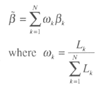
The weighting has been considered to give more importance to the regressions that are more likely to be close to the true model. The mean variance of the estimates is:

Under the hypothesis of Normality, having the mean and the variance, it is possible to compute the cumulative density function CDF and rely on the statistical tables to know the degree of significance of the regressors. The first thing to do then is to check if the hypothesis of normality of the distribution of β is plausible. For this we use the Shapiro-Wilk normality test. If this test rejects the hypothesis of Normality, we adopt the alternative solution proposed by the author:

For each regression, compute the area under the density function to the right of 0. We call it φ_zj(0). Then compute the aggregate CDF(0)¹⁹ of (that we call Φ(0) as the weighting average of the individual φ_j(0).

We consider the unweighted average too, to consider the possibility that some regressions might suffer of endogeneity and can be spuriously highly weighted. The average weighting is: