ARTÍCULO CIENTÍFICO

 

The semicontinous Reactor: Modeling, Simulation and Control
Part II Nonlinear Control

 

El reactor semicontinuo: modelado, simulación y control
Parte II Control no lineal

 

 

Rónanth Zavaleta Mercado

Member of the Academy of Sciences of Bolivia
Dean of the School of Engineering, Universidad Católica Boliviana San Pablo at La Paz.
ronanth.zavaleta@gmail.com

Recibido: 2 de febrero 2016
Aceptado: 25 de febrero 2016

 

 

---

Abstract: Conservation equations are applied to the Semicontinuous Reactor, also known as the Semibatch Reactor (SBR) for the isothermal, adiabatic and non-isothermal case, to generate the necessary differential equations for modeling and simulation. The resulting equations, expressed in terms of dimensionless normalized variables, are solved numerically for consistency testing by means of computer algebra software (Mathcad^®). The model is also expressed in terms of meaningful dimensionless groups of the Damköhler and Biot type. The consistent model is then simulated for typical combinations of operating parameters in preparation for process control and stability simulation and analysis.

The SBR is typically non steady, of relatively high operating costs and low throughputs. However high conversions can be achieved and good temperature control allows for the minimizations of unwanted side reactions by means of maintaining low concentrations of one of the reactants. This reactor is extensively used in the manufacture of high value added chemicals (fine chemicals) and in reactions where a careful control is mandatory, such as in the production of high explosives. It is used in case of multiphase reactions involving gas bubbling such as the production of mono, di and tri chlorobenzene.

Part I of this article is devoted to generating a robus t modeling and simulation tool for the SBR, while Part II explores its control and stable behavior.

Key words: Semicontinuous Reactor, Semibatch Reactor, SBR control, stable behavior of reactors.

---

Resumen: Ecuaciones de conservación se aplican al Reactor Semicontinuo, también conocido como el reactor por lotes Semibatch (SBR) para los casos: isotérmico, adiabático y no isotérmico; para generar las ecuaciones diferenciales necesarias para el modelado y simulación. Las ecuaciones resultantes, expresados en términos de variables normalizadas sin dimensiones, se resuelven numéricamente para las pruebas de consistencia por medio de un software de álgebra computacional (Mathcad^®). El modelo también se expresa en términos de grupos adimensionales significativos del tipo Damköhler y Biot. El modelo consistente, se simula para combinaciones típicas de los parámetros de funcionamiento en la preparación para el control de procesos y simulación de estabilidad y análisis.

El SBR es típicamente no constante, de relativamente altos costos de operación y bajos rendimientos. Sin embargo altas conversiones pueden alcanzarse y un buen control de temperatura permite la minimización de reacciones secundarias no deseadas por medio del mantenimiento de concentraciones bajas de uno de los reactivos. Este reactor se utiliza ampliamente en la fabricación de productos químicos de alto valor añadido (productos químicos finos) y en las reacciones donde un cuidadoso control es obligatorio, como en la producción de explosivos de alta potencia. Se utiliza en el caso de reacciones de varias fases que implican formación de burbujas de gas tal como la producción de mono, di y tri clorobenceno.

La Parte I de este artículo está dedicado a la generación de una herramienta de modelado y simulación robusta para el SBR, mientras que la segunda parte explora su control y el comportamiento estable.

Palabras clave: Reactor semi-continuo, reactor Semibatch, control de SBR, comportamiento estable de los reactores.

---

 

 

1. Basic Control Setup

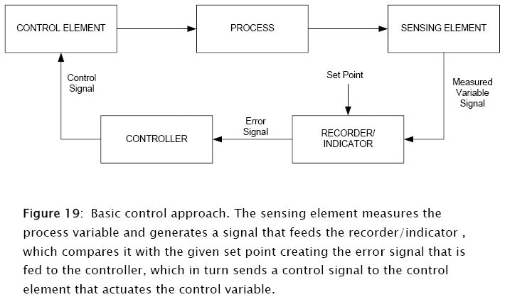
A basic traditional feedback configuration is used for the SBR reactor control, as depicted in the following Figure 18, which follows pretty much the approach due to R.G.E. Franks [1]. The sensing element measures the process variable and sends a signal to the recorder/indicator, which compares it with the given set point to generate an error signal that is in turn fed to the controller, which sends a control signal to the control element that in turn acts on the control variable (Figure 18:).

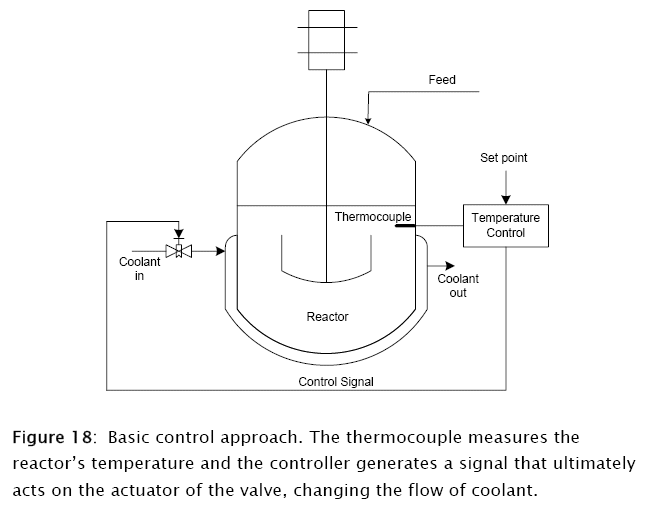
The control loop then consists of transfer functions, controls logic plus some instrumentation simulation (Figure 19:).

 

2. Modeling, transfer functions, control elements and controllers

In order to simulate the controlled behavior of the SBR, reactor the control elements must be modeled, including transfer functions for the sensing elements, controllers, actuators and valves. The software below simulates first and second order transfer functions, zero, one, two and three mode controllers (on-off, proportional, proportional-integral (PI) and proportional- integral with derivative action (PID)) as well as a generalized function for valve discharge.

2.1 Transfer functions

The first order transfer function is defined by a first order ordinary linear differential equation (ODE) with constant coefficients. In terms of Laplace transform notation

where G is the gain factor, τ the process time constant, V_0ut the output variable and V_in the input variable.

The following subprogram written in Mathcad Prime 3 software models the first order transfer function (TF1)

Subprogram 4: First order transfer function modeled as a first order linear ordinary differential equation with constant coefficients.

The second order transfer function is described by a second order ordinary linear differential equation (ODE) with constant coefficients. In terms of Laplace transform notation

where ζ, is the damping ratio. The corresponding subprogram for this second order transfer function (TFN2) is:

Subprogram 5: Second order transfer function modeled as a second order linear ordinary differential equation with constant coefficients. Here dout, the output variable derivative must be provided externally.

2.2 Control Elements

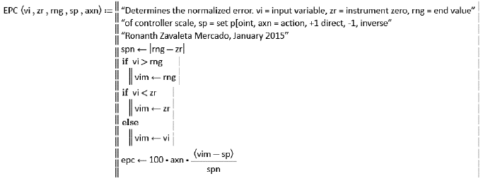
The following subprogram generates the normalized error EPC (with a domain from 0 to 100) obtained comparing the measured variable to the set point, and its corresponding limits. The general equation is:

where epc is the normalized percent error, axn the "action", direct or inverse, vi the measured input variable, sp the set point and spn the instrument span (difference between the range and zero of the instrument). The subprogram is displayed as Subprogram 6:.

Subprogram 6: Modeling of the normalized error. The input variable is vi, the set point sp, zr the zero of the instrument and rng its range and axn its "action", +1 direct, -1 inverse.

Since the SBR control, requires to modify the flow of coolant, it is necessary to simulate control valves. The most common of these control elements are the diaphragm or motor actuated control ones, that receive a signal coming out of the controller and converts it into a stem position that in turn control the port areas throttling the flow of coolant.

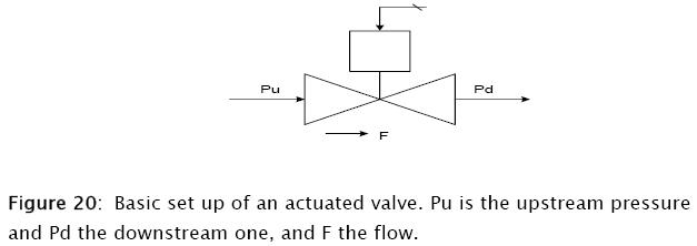
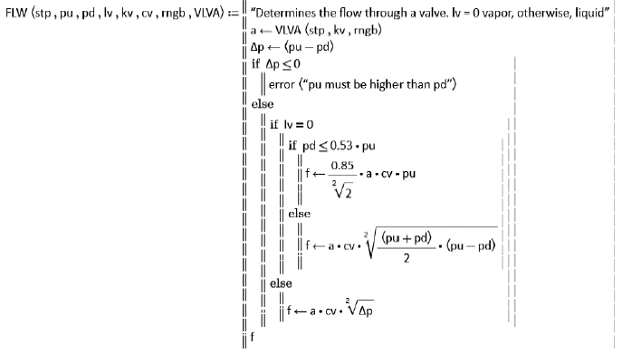
The flow of fluids through valves and restrictions is described by the following equation:

where A is the fractional valve opening, C_v the valve capacity, a function of the valve size and its service. It normally refers to the case when the valve opening is fully opened (A = 1), and subject to a unity pressure drop (P_u — P_d =1)- The pressure function f(P) depends on the phase of the fluid (whether liquid or gas), and sometimes on the flow characteristic (whether critical or subcritical). A typical approach is given below [2]

Another very important valve characteristic is the dependence of the port area on the stem position. This is a rather complex relationship and depends on the actual valve port characteristics, flow, pressure drop, turbulence and so on. Thus, the port area is expressed as the equivalent flow area rather than the actual geometrical one.

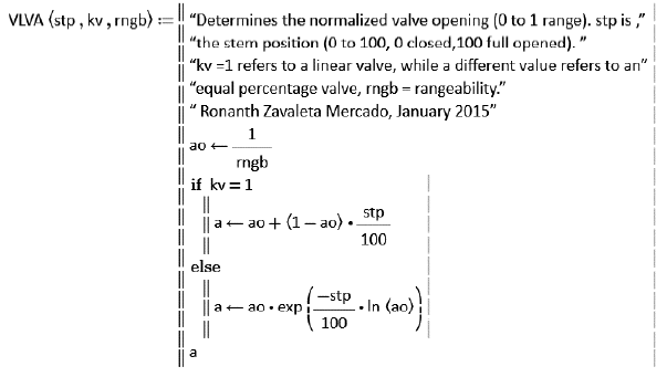
Two types of valves have been included in the simulation subprograms, a linear one and an equal percentage one. The first one gives a linear response of the port fractional aperture to changes in the valve stem position, and the second one provides a semilogarithmic one (Figure 21). Note the residual fractional port aperture when the valve is fully closed, aperture that corresponds to the "rangeability", the number of times the minimum residual flow may be increased before reaching the maximum flow. This is due to the fact of fabrication difficulties that make not practical to shut off a valve completely.

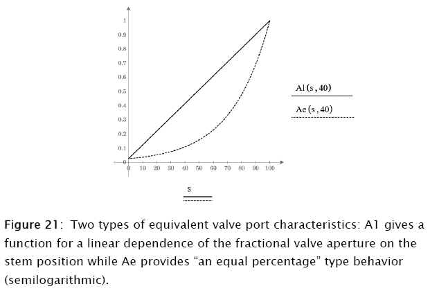
The two types of valve fractional aperture behavior are programmed in Subprogram 7:, and the associated flows (equations 69-71) in Subprogram 8.

Subprogram 7: Modeling linear and equal percentage valves: stp is the normalized stem position, kv an index that defines the port characteristics (1, linear, other, equal percentage) and rngb is the rangeability.

 

Subprogram 8: Modeling of the flow through the valve: stp is the stem position, pu the upstream pressure, pd the downstream pressure, Iv the phase indicator ( Iv = 0, vapor, other, liquid), kv is the port characteristic selector (kv=1, linear, other, equal percentage), cv is the valve capacity, rngb, the rangeability).

2.3 Controllers

The four basic industrial controller are modeled and simulated. These controllers include a) on-off b) proportional (P) c) proportional — Integral (PI) and d) proportional integral with derivative action (PID). The PI controller is sometimes referred as proportional with automatic reset, while the PID, proportional, reset with rate action.

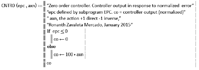
The On-Off controller is the basic form of control. Its logic is quite simple: whenever the controlled variable differs from the set point full action is imposed on the control elements, being this "fully open" or "fully closed" depending on the action of the controller. This controller is referred as being of zero order and is modeled and simulated in Subprogram 9.

Subprogram 9: Modeling of the zero order controller. Here epc is the normalized error and axn the action. The controller output co is also normalized (domain 0 to 100).

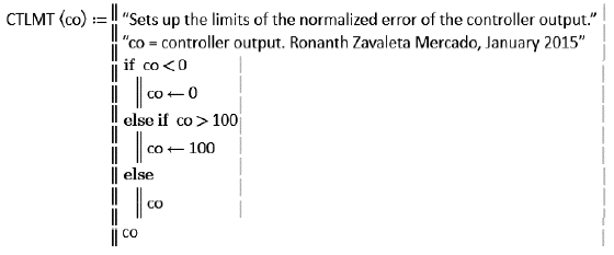
In order to simulate the remaining controllers, a subprogram for limiting the controller output to its domain must be developed. This is done in Subprogram 10 which is going to be called upon by the rest of the controller subprograms.

Subprogram 10: Limiting to its normalized domain the controller output (domain 0 to 100).

The first order controller (P) is based on the logic that the controller output co must be proportional to the normalized error epc. Therefore

where pb is the proportional band, axn is the "action" (direct or reverse) and oi is a manual reset, aimed at reducing the steady state offset. Subprogram 11 models this control controller (CONTR1).

Subprogram 11: Modeling of the first order controller. Here epc is the normalized error and oi the manual reset. The controller output co is also normalized (domain 0 to 100).

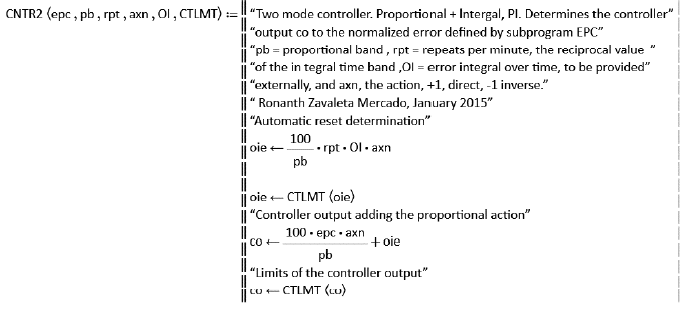
The second order controller, the proportional plus automatic reset one (PI) incorporates an additional action that is proportional to the integral of the normalized error, and its net effect is the elimination of the steady offset. It requires though the generation the integral of the error, function of time that has to be provided externally to the function CONTR2 that simulates it (Subprogram 12). The following equation describes this behavior

where rpt is the control setting that usually has units of repeats per minute [3].

Subprogram 12: Modeling of the second order controller (PI). Here epc is the normalized error and OI the integral over time of the error (epc) that has to be provided externally to the function. The controller output is also normalized (domain 0 to 100).

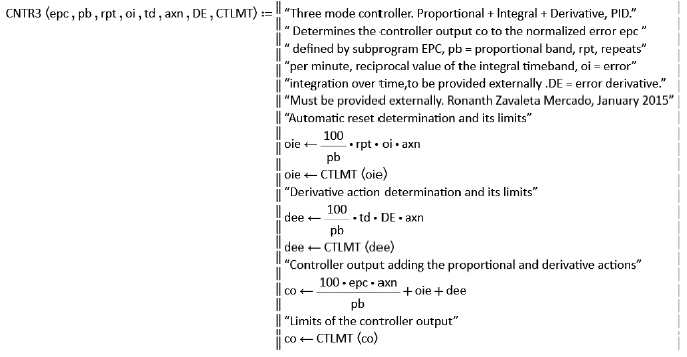
The third order controller (PID) incorporates a rate action to the PI controller already discussed and this way could be considered as some sort of a predictive one, since the rate action allows it to adjust a control variable according to the rate change of the error, before its build up. To model this controller not only the integral of the error has to be provided but also the rate of change of the error, that can be considered to be proportional to the rate of change of the control variable for a fixed set point (no servo control). This function of time has to be provided externally to the function CONTR3 that simulates it (Subprogram 13). The following equation describes this behavior.

Subprogram 13: Modeling of the third order controller (PID). Here epc is the normalized error, oi the integral of the error function epc, and DE the derivative of the control variable that has to be provided externals well. The controller output is also normalized (domain 0 to 100).

 

3. The nonlinear controlled SBR

The previously developed functions allow the simulation of the Semibatch Reactor by means of the mass and energy equations derived in the first part of this article. The case involving a second order elementary reaction is explored using proportional (P), proportional-integral (PI) and proportional-integral-derivative controllers (PID).

The following parameters were chosen for the simulation of the Semibatch reactor, and refer to the modeling presented in the first part of this article.

The resulting dimensionless groups for the mass and energy balances are

 

4. The non-adiabatic uncontrolled case

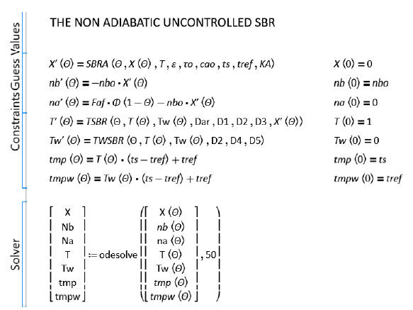
The application of the above parameters to the non-adiabatic uncontrolled SBR modeling (Subprogram 14, at the end) renders the results plotted in Figure 22. This data is displayed for comparison purposes with the controlled ones that are discussed below.

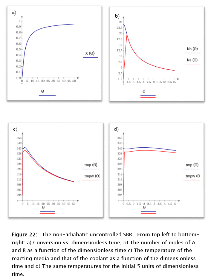
For this case the conversion tends asymptotically to 1 as expected for the irreversible second order elementary chemical reaction used, the number of moles of reactants follow a common monotonically decreasing behavior once the stoichiometric point is reached, also as expected. Both temperatures, reacting media and coolant, also follow this tendency, typical of the uncontrolled stable processes, with the coolant temperature lower than that of the reacting media.

 

5. The non-adiabatic controlled (proportional) case.

The following parameters were used for the proportional controller:

 

6. The non-adiabatic controlled proportional case.

The following parameters were used for the proportional controller:

and also the following function of the flow rate as a function of the port opening (valve area flow as a percentage of the fully opened one) and the corresponding dimensionless group

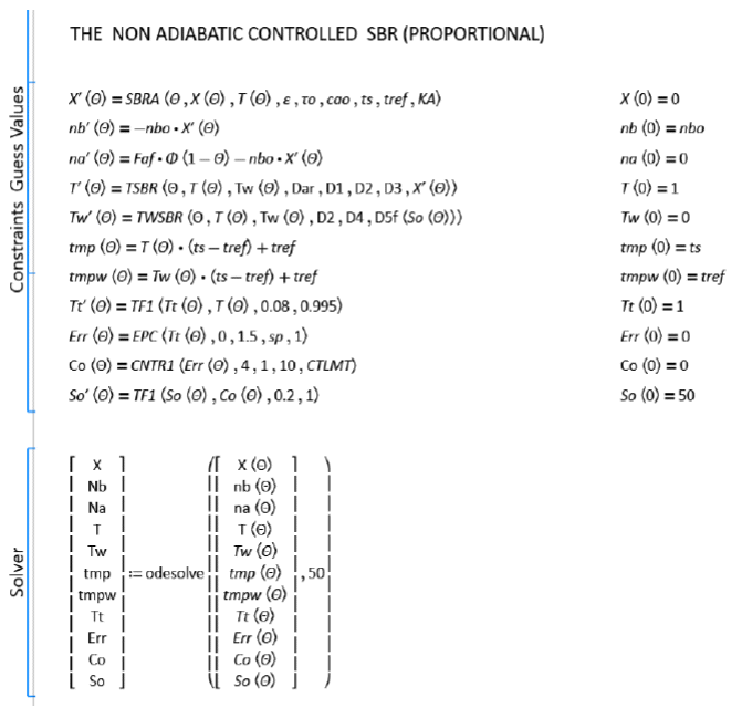
The application of the above parameters to the non-adiabatic uncontrolled SBR modeling (Subprogram 15) render the results plotted in figures 23 and 24

 

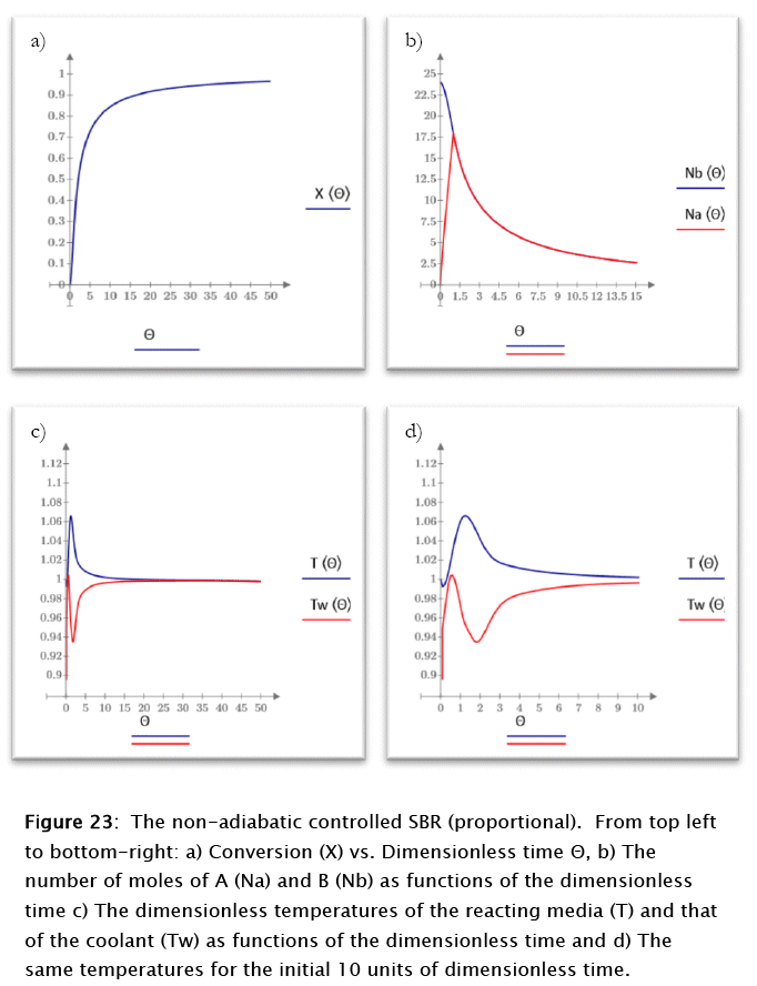
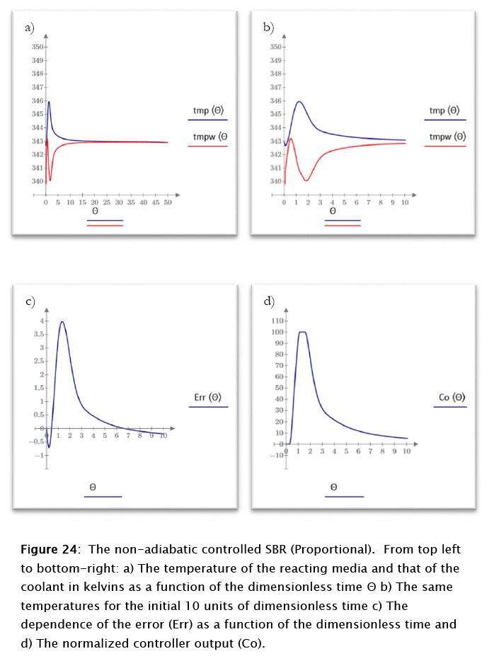
For this case the conversion and the number of moles of reactants follow patterns similar to the ones discussed above for the uncontrolled case even though the kinetics is faster, probably because of the temperatures being closer to that of the set point throughout the run, due to the controller activity, but the reacting media and coolant temperatures show a very different behavior. The reacting medium tend to reach the steady state value after an about 3 kelvins overshoot.

Close to steady state behavior is reached at about 20 dimensionless time units. The normalized error peaks at about 4 units for time 2 (dimensionless), in correspondence to the controller maximum output, as expected from theoretical considerations. A true steady state is never reached due to the residual coolant flow resulting from the valve's rangeability. The slight negative slope of the final reacting media and coolant temperatures results from this fact, as expected also from theoretical considerations.

 

7. The non-adiabatic controlled poportional-integral (PI) case.

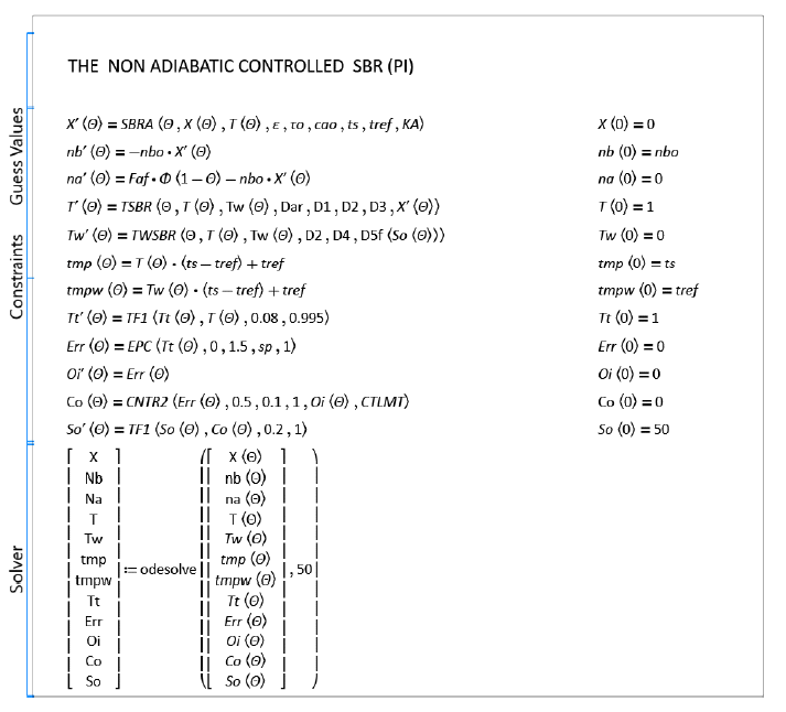
The parameters used for this case are the same ones discussed for the proportional controller, with the exception of those related to the settings of the controller itself, which are given as arguments of the function CONTR2 in Subprogram 16 (integral time and others).

The application of the above parameters to the non-adiabatic uncontrolled SBR modeling (Subprogram 16) renders the results plotted in figures 25 and 26

 

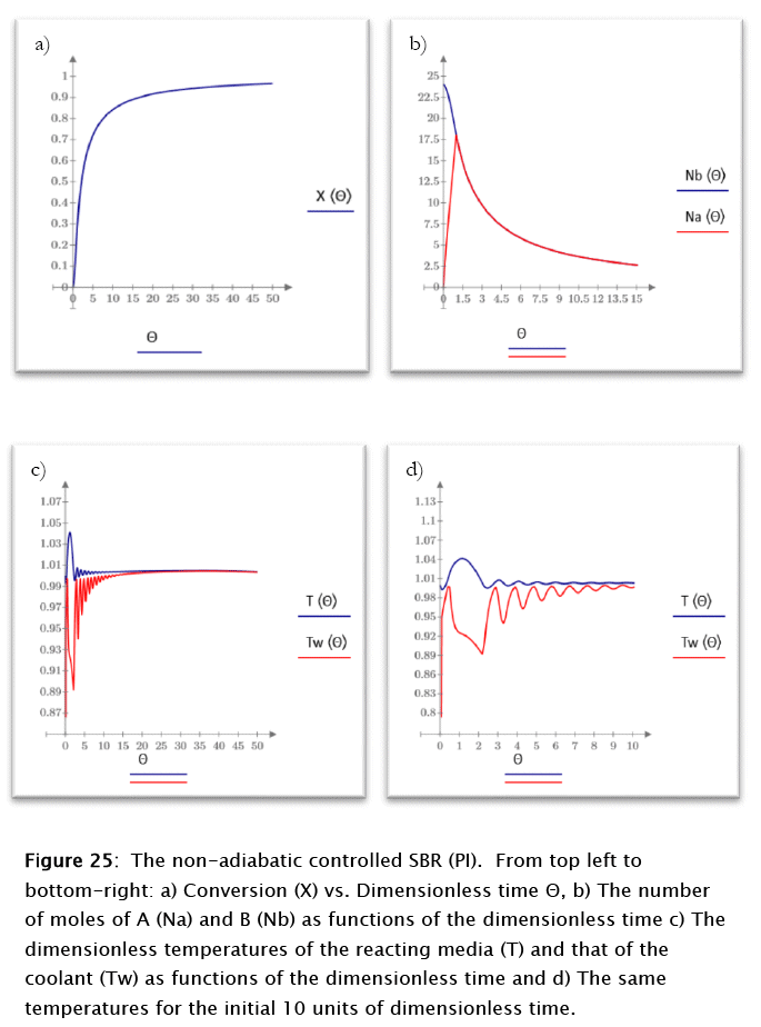
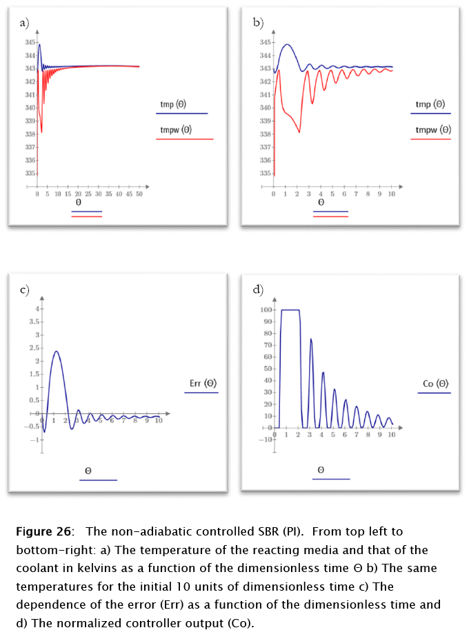
For this case the conversion and the number of moles of reactants follow patterns similar to the ones discussed above for the proportional case, but the reacting media and coolant temperatures show a very different behavior. The reacting medium tend to reach the steady state in time 9 (dimensionless) after an about 2.5 kelvins overshoot. The normalized error peaks at about 2.5 units for time 1.2 (dimensionless), in correspondence to the controller maximum output, as expected from theoretical considerations. A true steady state is never reached due to the residual coolant flow resulting from the valve's rangeability. The slight negative slope of the final reacting media and coolant temperatures results from this fact, as expected also from theoretical considerations.

In general the overall control of the process is greatly enhanced by the introduction of the integral effect.

 

8. The non-adiabatic controlled proportional-integral-derivative (PID) case.

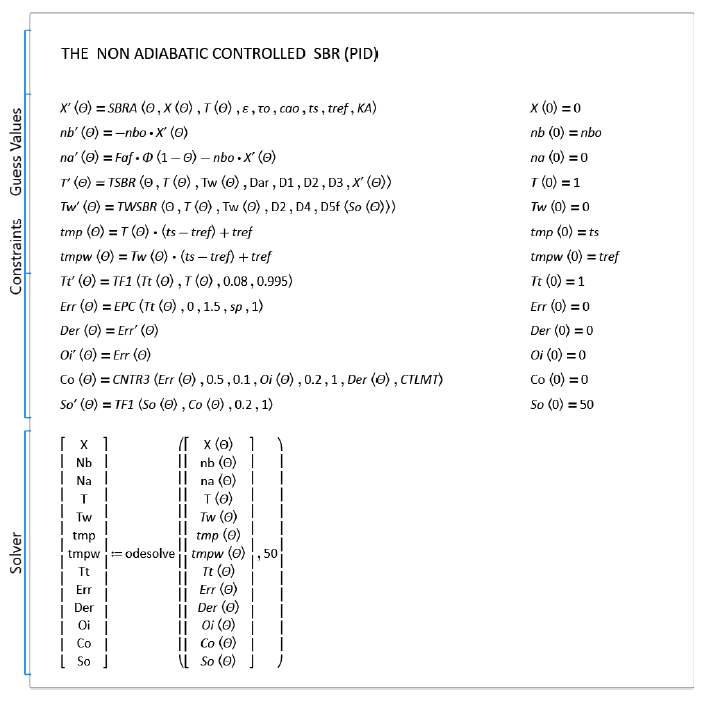
The parameters used for this case are the same ones discussed for the proportional controller, with the exception of those related to the settings of the controller itself, which are given as arguments of the function CONTR3 in Subprogram 17 (derivative time and others).

The application of the above parameters to the non-adiabatic uncontrolled SBR modeling (Subprogram 17) gives the results plotted in figures 27 and 28

 

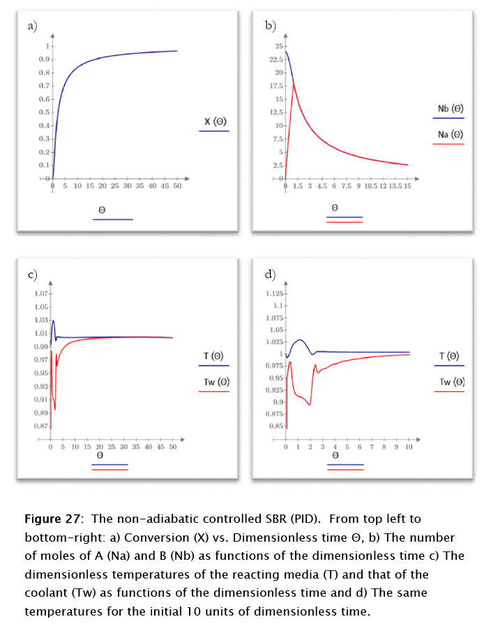
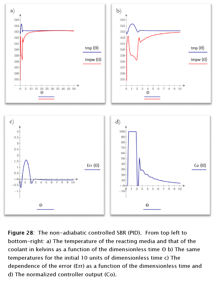
For this case the conversion and the number of moles of reactants follow patterns similar to the ones discussed above for the proportional-integral case, but the reacting media and coolant temperatures show a very different behavior. The reacting medium tend to reach the steady state after about 3 time units, following a 1 kelvin overshoot. The normalized error peaks at about 1.5 units for time 1.2 (dimensionless), in correspondence to the controller maximum output, as expected from theoretical considerations. As before, a true steady state is never reached due to the residual coolant flow resulting from the valve's rangeability. The slight negative slope of the final reacting media and coolant temperatures results from this fact, as expected also from theoretical considerations.

In general the control of the process is improved further by the introduction of the derivative effect, which provides a sort of predictive effect to the overall control.

 

9. Conclusions

The ease and versatility of functions manipulation of the Mead Prime 3 environment makes the control problem simulation studied a good experience. Even though no attempt was made to fine tune the controllers, the potential is there with little additional effort. Theoretical approaches for optimizing the process

are also possible employing real settings for the controller and control elements under an heuristic optimizing algorithm. Other more elaborate control schemes are also possible without having to endure complex programming.

In general the controllers performed as expected, and the real advantages of superimposing integral and derivative effects to the proportional controller become quite obvious for the case under study.

Subprogram 14: Modeling the non-adiabatic uncontrolled SBR. The results up to fifty dimensionless time units are portrayed in Figure 22.

Subprogram 15: Modeling the non-adiabatic controlled (proportional, P) SBR. The results are portrayed in Figure 23 and 24.

Subprogram 16: Modeling the non-adiabatic controlled (proportional, P) SBR. The results are portrayed in Figure 25 and 26.

Subprogram 17: Modeling the non-adiabatic controlled (PID) SBR. The results are portrayed in Figure 27 and 28.

 

Notation

Variables

A, B, C, D = chemical species A, B, C, D respectively. A refers also to the area available for heat transfer.

c = specific heat capacity

C = Heat capacity of the reactor contents

F = reactant feed rate

H = Enthalpy

n, N = number of moles

k = chemical reaction rate constant

r = chemical reaction rate

t = time

T = Temperature

U = Internal energy, also the global heat transfer coefficient

V = volume of the chemical reaction media

z = factor de compresion

Parameters

Da, Da_f = dimensionless Damkohler type parameters defined by Equation [48]

Da_r = another Damkohler type parameter defined by Equation [57]

D₁, D₂, D₃ = parameters for the energy balance defined by Equation [57]

Greek Letters

A = incremental operator, when referred to chemical reactions gives the enthalpy or internal energy of reaction

ρ = density of the chemical reaction medium

ε = ratio of the stoichiometric initial concentrations of species B in the reactor and A in the feed

Γ = Feed rate of reactant

ν = stoichiometric coefficient of an elementary chemical reaction.

9 = volumetric feed rate

X = chemical reaction conversion

Θ = dimensionless time

t = space time, also a dimensionless temperature

Subscripts

A, B, C, D = species A, B, C, D respectively

o, 0 = refers to a parameter at the beginning of the run

f = refers to a parameter at the end of the run and also to the feed

m = molar, specific property

ref = reference, used with T refers to a reference temperature

S = refers to the solvent

w = refers to the cooling medium

 

Bibliography

[1] Franks, R. G. E., "Modeling and Simulation in Chemical Engineering", Wile-Interscience, John Wiley & Sons, 1972

[2] Ibid, pg. 370

[3] Ibid, pg. 363