Inglés (pdf)
 Articulo en XML
 Referencias del artículo
 Enviar articulo por email
 Citado por SciELO
  Similares en
SciELO
Similares en
SciELO 
 Permalink
Classification/Clasificación JEL: F33, F41, F61, D12, O54.
Introduction
While currency crashes and large devaluations were once thought to be a thing of the past, Bolivia’s current currency crisis reminds us that those days are not gone. In 1985, following a severe economic crisis marked by hyperinflation, the government implemented a series of economic reforms to stabilize the economy, including a significant devaluation and the introduction of a floating exchange rate system de Bolivia (1985). However, in November 2011, the new government decided to return to a fixed exchange rate regime to:
encourage the use of the Boliviano over foreign currencies, strengthening monetary sovereignty. This helps stabilize domestic prices, prevents imported inflation, and creates a more predictable economic environment, which fosters confidence among investors and consumers.
While the fixed exchange rate contributed to price stability for a while, fluctuations in the international price of oil and erosion of Bolivia’s natural gas production and exports have reduced international reserves from a peak of almost US$15 billion to levels below US$1 billion, pushing the country towards a looming and old-fashioned currency crisis.
Plans to cut red tape and offer preferential exchange rates for exporters have not increased the flow of dollars into the economy. Government-imposed capital controls, including limits to the withdrawal of foreign currency, have increased devaluation expectations, creating a black market where a dollar is worth far more than its official value. As the spread between official and parallel exchange rates increases, importers experience higher marginal costs and a squeeze on their profits. Conversely, exporters see an opportunity to increase their profit by using higher black market exchange rates. Both factors contribute to reduced tax revenue from formal markets, further exacerbating government imbalances.
At the household level, devaluation has been passed through price increases in both foreign and local goods. Devaluation increased the marginal cost of imports, leading to price increases in foreign varieties. As some of these goods are inputs for goods produced at home, devaluation has also increased the marginal costs and prices of local varieties. Inflation tends to disproportionately hit lower-income households, eroding their purchasing power because they spend a large share of their budget on food. However, since high-income households usually spend a higher share of their budget on imported varieties, whose prices increase more in a devaluation, they may suffer more from higher inflation and experience a larger decline in their purchasing power. Yet, the final distributional effects of who bears the cost of devaluation depend not only on increases in the marginal cost but also on how firms adjust their retail margins, introduce new varieties, and how consumers substitute expensive products and varieties for cheaper ones.
This paper uses detailed scanner transaction data -at the product- variety level, from a major supermarket chain to analyze the consumer’s price and cost-of-living effects of the de facto exchange rate devaluation from January 2024 to January 2025. Assuming that more affluent consumers tend to purchase higher-priced products, we can categorize consumers by income strata based on their Engel curves. This allows us to explore the difference in cost-of- living effects for low- and high-income consumers. Observing prices, quantities, and costs for local and foreign varieties within narrowly defined product categories allows us to examine how price changes relate to changes in cost and retail margins and how currency devaluation affects product availability and substitution without imposing strong structural assumptions on the market structure.
We find that after a de facto devaluation, consumer prices rose, on average, by 12% after five months and by 16% after a year. Price increases were not uniform. Prices of foreign varieties increased by 17% during the first five months, to stabilize at 15% after a year. On the other hand, prices of local varieties increase by 9% after 5 years, during the first five months, to stabilize at 16% after a year.
Since significant differences exist in expenditure shares within detailed product categories across income strata, with high-income consumers allocating a larger share of their spending to foreign varieties relative to low-income consumers, we expect high-income consumers to suffer higher cost-of-living effects. However, decomposing changes in the cost of living into markup, cost, substitution, and variety channels allow us to report that the firm reduction of retail margins, consumers’ ability to reallocate spending substituting expensive products; and the entry and exit of different varieties reduce the cost of living effects of devaluation for high-income consumers to levels that are lower than those observed for their low-income counterparts who face unchanged margins, lower elasticities of substitution and no new entries in the varieties they consume.
Using detailed consumer-level price and quantity data, our work contributes to the literature examining the impact of currency crises on consumer price levels, cost of living, and overall income distribution. Prior research has explored various channels through which currency crises affect price dynamics, including retail margins, product variety, and the pass- through of prices.
There is significant evidence suggesting that retail margins play a crucial role in explaining the disconnect between consumer and border prices (Burstein et al., 2003; Hellerstein, 2008; Berger et al., 2012; Gopinath and Itskhoki, 2011; Alessandria et al., 2019; Auer and Tille, 2021). However, much less is known about how these margins adjust in response to international shocks, particularly whether changes in distribution margins mitigate relative price adjustments following currency devaluations. Studies have shown that firms adjust margins strategically depending on demand elasticity, local competition, and the degree of import penetration (Campbell and Lapham, 2019; Amiti et al., 2020).
The role of product variety in price adjustments is also critical. In a closed-economy context, less appealing products are frequently replaced by more desirable ones, mitigating inflationary pressures (Bernard et al., 2010; Broda and Weinstein, 2010; Argente and Lee, 2024). This variety effect has been shown to play a substantial role during economic downturns. For instance, Argente and Lee (2021) found that the variety channel dampened the cost of living for all US income groups during the Great Recession by enabling substitution toward newer, more appealing product varieties. Additionally, product assortment adjustments influence price pass-through, as firms alter product availability to maintain competitiveness in response to exchange rate fluctuations (Nakamura & Steinsson, 2014; Caballero, & Krishnamurthy, 2004; Goetz & Rodnyansky, 2019; Gopinath et al., 2017; Christiano et al., 2004).
By building on these insights, our study contributes to the growing body of literature on the transmission mechanisms of currency crises to consumer prices, retail margins, and adjustments in product variety. The remainder of the paper is organized as follows. Section 2 describes the Bolivian currency crisis. Section 3 presents the data and analyzes the effects of devaluation on prices. Section 4 presents our approach for estimating the cost of living effects of devaluation and decomposed into (1) a marginal cost, (2) a retail markup, (3) a substitution channel-capturing consumers’ ability to reallocate spending, and (4) a variety channel-capturing the introduction of new cheaper varieties. Section 5 uses these results to report some microsimulation exercises that examine the changes in the full income distribution due to devaluation and their consequences for poverty and inequality. The last section concludes with a review of our main results and a discussion of policy alternatives.
Bolivia’s Current Currency Crisis
Bolivia is a small emerging economy that primarily relies on commodity exports, especially natural gas, and takes global prices as given. A change in government and favorable economic conditions prompted the implementation of a fixed exchange rate regime. Since 2008, the Boliviano has been pegged to the US dollar at 6.86 for buying and 6.96 for selling. The success of this fixed exchange rate policy has heavily depended on gas exports. However, a decline in international crude oil prices, a sustained reduction in domestic production in 2015, and an expansionary fiscal policy that included debt monetization have created significant pressure on the country’s foreign reserves.
Figure 1 illustrates the evolution of Bolivia’s total foreign reserves, showing both the absolute values and year-to-year changes (panel a) alongside international oil prices (in US$ per barrel) and local production (in thousands of barrels per day). From the mid-2000s to their peak in 2015, which coincided with historically high international oil prices, Bolivia’s foreign reserves experienced a sharp increase driven by hydrocarbon exports, particularly natural gas. However, following the global oil price crash in 2015, reserves declined rapidly. Even after oil prices rebounded in 2017, reserves continued to fall due to significant and ongoing reductions in oil production and export revenues. Local production decreased from a peak of 62,000 barrels per day in July 2015 to a low of 19,000 barrels per day in September 2024.
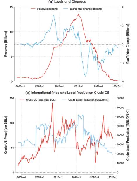
The significant decline in reserves has weakened public confidence in the fixed exchange rate. By 2024, Bolivia’s reserves had fallen to critically low levels, placing the Central Bank in a challenging position to maintain the currency peg. As suggested by currency crisis models, such as those by Krugman and Obstfeld, the low reserves and macroeconomic imbalances have heightened expectations of devaluation. This increased the currency crisis risk, leading to speculative attacks on the Boliviano.
The government has implemented policies to address the dollar shortage and encourage the inflow of foreign currency. In February 2023, the Banco Central de Bolivia (BCB) offered exporters a preferential exchange rate of 0.09 Bolivianos, higher than the official rate. However, rather than attracting dollars from private exporters as intended, this policy highlighted the strain on the fixed exchange rate system. It led to increased expectations of currency devaluation, heightened demand for dollars, increasing capital outflows, and further declines in foreign reserves. In July 2024, the government implemented strict measures to regulate access to US dollars and limit foreign currency withdrawals from banks (Digital, 2024). These measures included a daily withdrawal cap of US$100 at most banks. Additionally, there were restrictions on international transactions, allowing online purchases of up to US$100 per week and limiting foreign transactions made with debit and credit cards to between US$300 and US$1,500 per month.
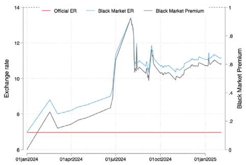
The persistent shortages of dollars and strict capital controls have forced individuals and businesses to rely on black markets and a dual exchange rate system. In this system, different segments of the economy access foreign currency at varying rates. Figure 2 illustrates the evolution of Bolivia’s official and black market exchange rates from January 2024 to January 2025. The official exchange rate (indicated by the red line) remains pegged at 6.96 bolivianos per US dollar, while the black market rates (shown by the blue line) have steadily increased throughout the year. Aher experiencing a significant spike, the black market premium reached a peak of almost 100% above the official rate. By January 2025, the unofficial rate has stabilized, maintaining a premium of around 60%. As suggested by Drazen (2000), political instability and the upcoming 2025 elections have delayed formal devaluation, leading to increased political uncertainty and a decline in investor confidence.
Source: Author’s compilation.
Figure 2: Official & Black Market Exchange Rates and Premium. January 2024 to January 2025
Notes: Data sourced from Reuters. “Bolivia unveils measures to tackle sharpening dollar crisis”, February 20, 2024. OPB. “Economic turmoil in Bolivia fuels distrust in government and its failed coup claim”, July 1, 2024. GIS Reports. “Bolivia’s political chaos puts the economy at risk”, August 2024. Reuters. “As Bolivia’s big state economic model slowly implodes, fear of ’total crisis’” December 16, 2024. Binance. “Bolivian Boliviano to US Dollar Exchange Rate”, February 2025.
The ongoing de facto devaluation of the Boliviano from January 2024 to January 2025 presents an interesting case for examining how exchange rate shocks affect consumer prices and the cost of living, allowing us to identify a clear pre- and post-devaluation period.
Pass-through Effects
Data
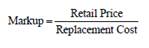
We use detailed consumer purchase data collected through daily price scans at the variety/ product level from a large chain of supermarkets. The data cover all stores in the three main cities of Bolivia (La Paz, Cochabamba, and Santa Cruz) and span the period from January 02, 2024, to January 31, 2025. Along with the store location, timestamp, an anonymized customer ID based on customers’ tax ID information (Numero de Identificacion Tributaria (NIT)), quantities, and prices for each item purchased, we also have inventory data. Inventory records enable us to calculate variety-level replacement costs using a first-in, first-out (FIFO) inventory system. We compute retail markups as
Consumer’s Selection
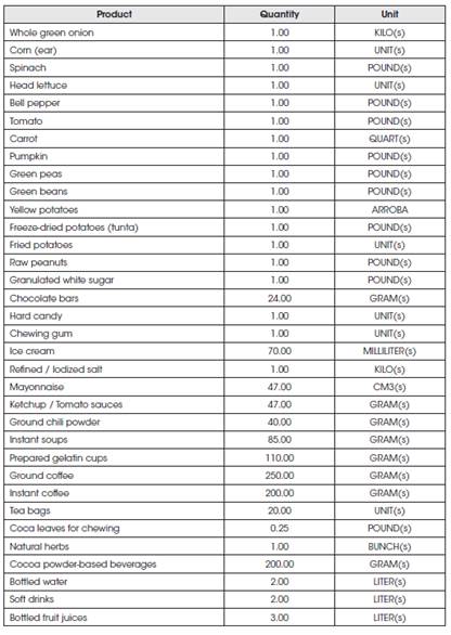
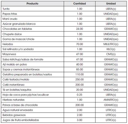
Our database includes households and small business owners, such as restaurants and small shops. To filter out small business owners, we exclude transactions with unusually high expenditures, which are unlikely to be made by households. Table 1 presents the monthly spending by per capita income percentile. We take the 99th percentile per capita income expenditure as the relevant cutoff value.
We restrict our sample to frequent shoppers. We use the customer’s unique tax ID to track individual transactions and limit the sample shoppers to those with a shopping history for at least 7 of the 13 available months. Observing the same consumer over time reduces potential biases from sample attrition.
Table 1 Average Monthly per-capita Income and Annual Food Household Expenditure for 2024 (In Bolivianos of January 2024)
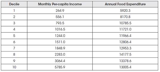
Source: Author’s calculation based on the nowcasted 2023 Household Survey integrated with the nowcasted 2016 Household Budget Survey.
Notes: To update the 2023 data to 2024, we assume neutral per capita income growth. To integrate the 2016 food share, we use random forest prediction based on jointly observed household characteristics and budget share statistics.
Product’s Selection
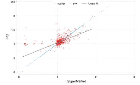
Our dataset covers the full range of products available at the store, including food, non-alcoholic beverages, alcoholic beverages, tobacco, cleaning items, cooking supplies, and clothing. Our analysis focuses only on the information for food and beverage items because only these items exhibit a comparable price trajectory to that observed in the Consumer Price Index (CPI). Figure 3 compares the price change between January 2024 and January 2025 for the three main cities of Bolivia of different product categories relative to their CPI components. Price changes for food and beverage items in our scanner database are similar to those observed in the Consumer Price Index (CPI). The correlation is above 2/3, and inflation in supermarkets explains more than 44% of the variation of inflation in food and beverage items in the CPI.
Source: Author’s calculation based on scanner transaction data and CPI data at the product level.
Figure 3: Comparison of Observed Price Changes with CPI estimates. January 2024 to January 2025.
Notes: The figure plots observed price changes from our scanner transaction data with reported price change from the CPI provided by the NSO.
Within the food and beverage category, we follow the National Statistics Office classification and define three a subcategory level [“Clase”] (e.g., bread & cereals), a product group level [“Subclase”] (e.g., pork meat), and a product variety level (e.g., ground pork beef ). Product varieties were classified as foreign or local based on the barcode system1.
Income Classification
Ideally, consumer segmentation would be based on reported income, but this information is unavailable in our database. One approach would be to classify consumers based on total expenditure per capita. However, since we do not observe household size, it is unclear whether higher expenditure reflects higher income or a larger household size. As a result, we prefer to classify consumers using quality Engel curves. Quality Engel curves infer income levels from consumption patterns, assuming that, within product categories, wealthier consumers tend to purchase higher-priced varieties (Deaton, 1988; Bils & Klenow, 2001)2.
To avoid bias in income classification due to inflationary effects due to devaluation, we use only the first month a consumer is observed in our data to classify their income group based on the following procedure: First, we calculate prices in standardized units (e.g., Boliviano per ml or kg), ensuring product comparability. Second, within each product group, we rank varieties by their median pre-devaluation unit price and classify them into four quartile-based price categories:
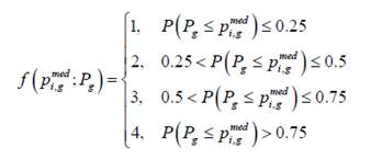
where p 𝑖,𝑔 𝑚𝑒𝑑 is the pre-devaluation median unit price of variety 𝑖 in product group 𝑔, and 𝑃 ?? is the distribution of pre-devaluation prices. Finally, we compute an expenditure-weighted index of the average price level of a consumer’s basket,
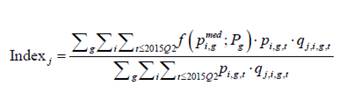
Consumers in the first quintile of this index distribution are classified as low-income, while those in the fifth quintile are classified as high-income.
Hedonic Price Regressions
To estimate the devaluation pass-through effect on consumer prices of food and beverage items, we use a simple hedonic price regression:
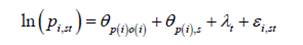
where ln 𝑝 𝑖,𝑠𝑡 is the natural logarithm of the consumer price of a variety 𝑖 in a store 𝑠 at time 𝑡, and 𝜆 𝑡 are time-fixed effects that highlight the inflationary consequences of the devaluation - relative to January 2024 (the excluded period). Our specification captures only short-run responses to shocks and ignores dynamic responses. To control for persistent price differences across the origin of the variety - i.e., imported products having higher prices relative to locally produced products, we include product-origin fixed effects 𝜃 𝑝 𝑖 𝑜 𝑖 . We include product-store fixed effects, 𝜃 𝑝 𝑖 ,𝑠 , to control for persistent differences across locations within product categories.
Overall Price Effects
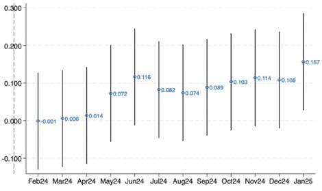
Figure 4 plots the estimated average time effects (λt) of currency devaluation on consumer prices from January 2024 to January 2025, with whiskers representing 95% confidence intervals around the point estimates computed from standard errors, clustered at the product- store level. Although no formal devaluation has been announced, the weakening of the local currency on the black market has increased overall inflation, despite government interventions such as food subsidies and price controls. The effects of devaluation on consumer prices have increased continuously following the devaluation trajectory. At the beginning of the crisis, the price impact was minimal and statistically insignificant until April 2024. The effect became large and statistically significant in May 2024, with a local high in June 2024 (a quarter before the exchange rate overshoot in August 2024) and a continuous increase, reaching 15.7% in January 2025, the highest point observed during our analysis period. Three points are essential to notice. First, price increases are leading changes in the exchange rates, which is consistent with a forward-looking pricing strategy. Therefore, if expectations of devaluation change, prices are likely to continue rising until the exchange rate reaches an equilibrium level. Finally, the relatively low pass-through effect of devaluation on average prices can be explained in part by several food subsidies (particularly for wheat) and price controls established at the national level, as well as in some cases at the local (municipal) level.
Differences by Product Origin
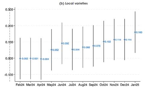
Figure 5 reports estimated time effects of devaluation on consumer prices from January 2024 to January 2025 from a hedonic price specification distinguishing between foreign and local varieties. Foreign varieties exhibit stronger and faster effects, while local products demonstrate a delayed but eventual increase, possibly due to the higher costs of imported inputs.
For foreign products, the coefficients show an early and steep price increase, with a peak value of 16.8% in June 2024, consistent with direct and forward-looking import price transmission of devaluation on imported goods. Aher the anticipated overshoot, the pass- through effect on foreign varieties stabilizes in the later months, around 9 to 11%, to increase again to a lower high level of 15.1% by January 2025.
On the other hand, the price increase for local products was initially lower but reached a higher level by the end of the period. Aher showing zero and statistically insignificant coefficients during the first month, prices increased, reaching a local high of 9.2% in June 2024. Aher reducing to 5.4% in the next month, it increased steadily to reach 16.0% in January 2025. These higher and somewhat delayed effects of devaluation may be associated with lagging and indirect impact through input costs due to higher imported inputs. The differential and asymmetric price responses of foreign and local varieties highlight compounding inflationary pressures across product origins, with leading and direct price responses from foreign varieties that reinforce lagging and indirect price responses from local varieties.
Source: Author’s calculation based on scanner transaction data at the product level from major supermarket chains.
Figure 5: Time Effects of devaluation on Consumer Prices, By Origin. January 2024 to January 2025
Notes: The figure plots λ coefficients which are obtained from hedonic price regressions. Coefficients are normalized relative to January 2024. Whiskers are 95% confidence intervals around the point estimates computed from standard errors, which are clustered at the product-store level. Foreign and local varieties are defined based on the barcode system.
Differences by Income Stratum
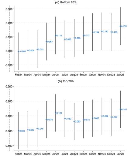
Figure 6 presents the pass-through effect for low-income consumers (bottom 20%) and high-income consumers (top 20%). As we explained, consumers’ income strata are classified into different income strata according to quality Engel curves. Low-income consumers’ price effects overshoot to 12.0% in June 2024, to stabilize between 7 and 9% in the next month, and reach a peak at 14.5% in January 2025. In contrast, the high-income consumers’ price effect overshoots to only 11% in June 2024, falls to 8.3% the next month, and then continuously increases to 17.6%. The fact that price increases are higher for low-income consumers at the beginning but are higher for higher-income consumers is consistent with a scenario in which lower-income consumers purchase a relatively larger share of imported goods, making them more sensitive to currency devaluation. The delayed but higher price effect for goods consumed by higher-income consumers suggests a greater reliance on locally produced goods. The lead price effect for goods consumed by lower-income consumers indicates that they are the first to be affected by devaluation due to their dependence on imported goods.
Source: Author’s calculation based on scanner transaction data at the product level from major supermarket chains.
Figure 6: Time Effects of devaluation on Consumer Prices, By Income Stratum. January 2024 to January 2025
Notes: The figure plots λ coefficients which are obtained from hedonic price regressions. Coefficients are normalized relative to January 2024. Whiskers are 95% confidence intervals around the point estimates computed from standard errors, which are clustered at the product-store level. Income strata are defined based on quality Engel curves.
Differences in Food Expenditure across Income Strata
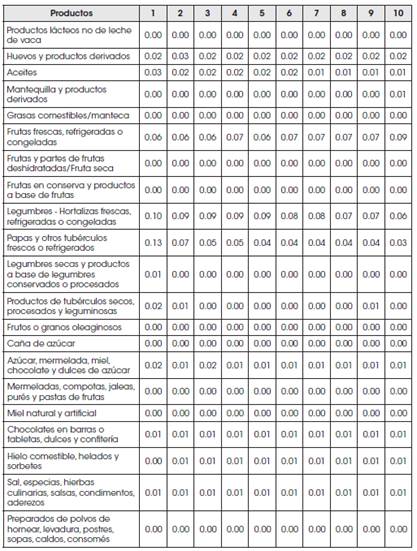
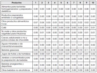
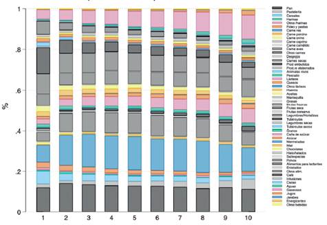
To confirm whether the poor rely more on imported goods, we use the 2016 Household Budget Survey to analyze the changes in food budget shares across income groups. Here, income groups are defined by per capita household income. Figure 7 presents the budget allocation for different food and beverage categories across income deciles. Product categories include staple foods (e.g., bread, cereals, pasta, and flour), protein sources (e.g., beef, pork, poultry, and fish), dairy and oils (e.g., milk, eggs, and oils), fruits and vegetables (e.g., fresh fruit, legumes, and vegetables), sugary products and processed foods (e.g., sugar, chocolates, fruit juices), and beverages (e.g., water, soh drinks, energy drinks, and infusions).
Notice that lower-income deciles (1st to 3rd) allocate a significant fraction of their food expenditure to staples (including bread, cereals, flour, and pasta), sugary products, and processed foods. In contrast, more locally produced foods, such as animal protein sources (especially beef, poultry, and pork), dairy products, processed meats, or fresh produce, account for a smaller share of their budget. In contrast, higher-income households (deciles 8th to 10th) exhibit a more diverse food basket, allocating a lower share of expenditure to staples, and a higher share of spending to higher-value foods, including meat, dairy, and fresh produce; and luxuries, premium or non-essential goods such as chocolates, honey, bottled water, and juices -which are relatively insignificant in the budgets of lower-income households.
Two key differences are worth noting. First, while we do not have the origin of the products in the Household Budget Survey, it is safe to assume that low-income households have a higher reliance on essential imported products where domestic production is insufficient or more expensive for consumers. This includes mainly staples, including rice, wheat and wheat- based products, pasta, and potatoes, which meet the demand for bread and other wheat-based products; processed foods3. On the other hand, high-income households allocate the largest share of their food budget to locally produced products such as protein sources (e.g., beef, pork, poultry, and fish), dairy and oils (e.g., milk, eggs, and oils), and fruits and vegetables (e.g., fresh fruit, legumes, and vegetables). Imported varieties are also important, but they are more related to non-essential luxury and premium items, such as spices, coffee, chocolates, or seasonal fruits.
Source: Author’s calculation based on Household Budget Survey 2019.
Figure 7: Budget Share of Food and Beverage Categories by Decile of Per-capita Household Income
Notes: The figure shows the budget share of different expenditure categories by decile of per capita household income. Each vertical bar corresponds to a particular decile (from 1 to 10 along the horizontal axis), and the stacked sections within each bar indicate the share of food and beverage expenditure devoted to a specific food category within that decile.
These findings will be key to explaining why we observe compensatory effects of the marginal cost increase, including reduced markups, higher substitution, and changes in variety effects, among high-income consumers but not among low-income consumers. While the rich can switch to cheaper varieties of luxury or premium goods, such as local chocolates instead of imported ones, the poor can substitute imported wheat or pasta if local varieties are unavailable or more expensive. Furthermore, as we will see in the next section, given that the rich can substitute, firms (and sellers) of imported goods find it more profitable to reduce their retail margins and absorb part of the marginal cost increase to keep at least part of the sales volume from dropping. On the other hand, staples such as wheat, wheat-based products, pasta, beans, or potatoes are necessities for the poor. Since they cannot substitute them, sellers can pass on most of the increase in marginal cost.
Cost of Living Effects
We approximate the cost of living effects by the household compensating variation, CVh, which is the amount of income required to maintain the household’s utility unchanged in response to the price changes induced by devaluation. In other words, it is the amount of income that would compensate for the change in the cost of living.
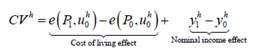
where 𝑒 ⋅ is the unit expenditure function that depends on the price vector at period 𝑡, 𝑃 𝑡 , and the utility of household ℎ at period 𝑡, 𝑢 𝑡 ℎ .
Notice that in addition to the cost of living effect -the pass-through impact of devaluation through inflation, there are also nominal income effects- a change in earnings for households that produce local varieties or trade foreign varieties informally. This paper focuses on changes in the cost of living, abstracting from the analysis of changes in nominal income.
Preferences
To obtain a closed-form solution for the expenditure function, we follow the literature [Colicev et al. (2024), (Atkin and Donaldson, 2018; Jaravel, 2019a; Argente et al., 2021)] and model consumer preferences using a nested mixed-CES demand system. The nested mixed-CES demand system is helpful because it captures preference heterogeneity by allowing budget shares and elasticities of substitution to vary across income groups [(Atkin et al., 2018; Jaravel, 2019b; Argente and Lee, 2021)]. Furthermore, it will enable heterogeneity on empirical estimates of the elasticities of demand by income groups that allow us to decompose the total cost of living effect into a price channel that can be further decomposed into changes in markups and marginal costs [(Redding and Weinstein, 2020)]; a variety channel - that capture the impact of product entry and exit on consumer welfare [(Feenstra, 1994; Broda and Weinstein, 2006)]; and a substitution channel. The nested mixed-CES demand structure allows for substitution across two nests: An upper nest that captures substitution across products (e.g., rice vs. potatoes), and a lower nest -defined at the variety level that captures substitution across varieties within the same product (e.g., imported rice vs. national rice). After devaluation, substitution between products is determined by the elasticity of substitution between products, 𝜎 ℎ . For example, if devaluation causes bread prices to increase relative to rice, consumers might substitute bread for rice. The product level is the finest level of aggregation, where there is no meaningful product entry or exit after devaluation. In contrast, varieties’ entry or exit is determined by the elasticity of substitution across varieties, 𝜂 𝑝 ℎ .
In the upper nest, the CES aggregator is given by:
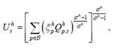
where 𝑄 𝑝,𝑡 ℎ is the aggregate consumption of product 𝑝 by households in income group ℎ at time 𝑡. - 𝜉 𝑝 ℎ is a product-level demand shifter, which may differ across income groups. - ℬ is the set of available products. - 𝜎 ℎ is the elasticity of substitution across products.
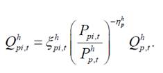
At the lower nest, the product-specific quantity, 𝑄 𝑝,𝑡 ℎ , is itself a CES aggregator over individual varieties given by:
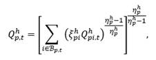
where 𝑄 𝑝𝑖,𝑡 ℎ is the consumption of variety 𝑖 by households in income group ℎ at time 𝑡, 𝜉 𝑝𝑖 ℎ is a variety-level demand shifter, and 𝜂 𝑝 ℎ is the elasticity of substitution between varieties of product 𝑝.
In the Nested-CES framework, consumers of the same income group share the same elasticity of substitution across foreign and local varieties. Local and foreign varieties compete within highly detailed product categories and face the same elasticity of substitution within income groups. Yet, it allows for differences in preferences between foreign and local varieties between rich and poor consumers.
Given this preference structure, the category-level and product-level unit expenditure functions are given, respectively, by
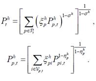
where 𝑃 𝑝𝑖,𝑡 ℎ is the price of variety 𝑖 at time 𝑡.
Decomposition of the Cost of Living Effect
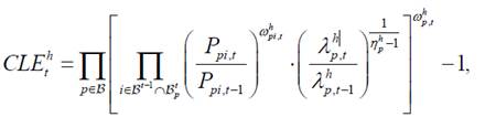
The cost-of-living effect of consumer h can be broken down into three channels: A price channel, that includes a marginal cost effect and a markup effect; a substitution channel, that captures consumer responses to relative price changes; and a variety channel, that captures the impact of changes in available varieties.
Since the income-group-specific utility functions are homothetic, the change in the cost of living is equivalent to the change in the unit expenditure function. That is,

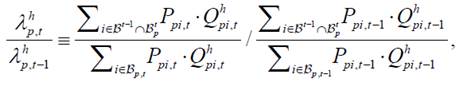
where 𝜔 𝑝,𝑡 ℎ are the Sato-Vartia weights4
The change in the product-level unit expenditure function can be further decomposed into a term that depends on variety-level price changes for continuing products and a term that captures changes in product availability (Feenstra, 1994):
where 𝜔 𝑝𝑖,𝑡 ℎ are the variety-level Sato-Vartia weights5
The variety effect will be given by,
Finally, using the definition of retail markups, 𝑃 𝑝𝑖,𝑡 ≡ 𝑀 𝑝𝑖,𝑡 ⋅ 𝐶 𝑝𝑖,𝑡 , the ratio of the final consumer price to the marginal cost,
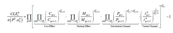
The price channel is the covariance between pre-devaluation expenditure shares of continuing varieties and changes in consumer prices. If different income groups have different expenditure shares on other varieties, we will expect differential effects on the cost of living. For example, if affluent consumers spend relatively more on foreign varieties, and if foreign varieties experience a greater price increase, the price channel will increase more for rich consumers.
The price channel can be further decomposed into a cost effect associated with changes in marginal costs, and a markup effect related to changes in retailers’ margins (Borusyak et al., 2018; Fajgelbaum, & Schaal, 2019). If rich consumers had larger pre-devaluation expenditure shares on foreign varieties, we would expect relatively larger increases in the cost of living for rich consumers due to changes in the marginal cost. However, if the elasticity of substitution is high, profit maximization predicts that firms will decrease their retail margins, offsetting increases in the marginal cost.
The substitution channel is the covariance between changes in final consumer prices and the difference in variety-level Sato-Vartia weights and variety-level pre-devaluation expenditure shares. If consumers reallocate expenditure away from varieties with higher price increases, their post-devaluation increase in the cost of living will be lower. If high-income consumers have higher elasticities of substitution, we would expect stronger substitution away from varieties with higher price increases for them, which would attenuate their increase in the cost of living. As emphasized by Auer et al. (2023), it reflects consumer adjustment behavior in response to price changes.
Finally, the variety channel captures how changes in product availability (the so-called extensive margin) affect consumer cost of living. It comprises the ratio of the expenditure share on continuing varieties before and after the devaluation, along with the variety-level elasticity of substitution. If the ratio of expenditure shares is below one, the appeal of the varieties that entered must have been greater than that of the varieties that exited. The extent to which this reallocation of expenditure translates into changes in the cost of living depends on the elasticity of substitution. The distributional cost-of-living effects of the variety effect depend on the difference in the elasticity of substitution across income groups. If the elasticity is high, products are perceived as good substitutes, and adding new varieties increases utility only marginally.
Quantifying Changes in the Cost of Living
To analyze changes in the cost of living, we need to obtain a functional form for the residual demand of variety i and derive a form that allows us to estimate the variety-level elasticities of substitution. Using Shephard’s lemma,
Taking logs,
where lowercase variables indicate their logarithmic transformations and 𝜂 𝑝 ℎ is the elasticity of substitution. Consistent estimation of these parameters requires overcoming several econometric challenges. First, there is a simultaneity problem between product-level price, 𝑃 𝑝,𝑡 ℎ , and quantity, 𝑄 𝑝,𝑡 ℎ , since both indices depend on unobserved demand shifters. To mitigate this, we include product-income-time fixed effects.
Second, since demand shifters 𝜉 𝑝𝑖,𝑡 ℎ are unobserved. If firms anticipate these demand shifters, they may set prices with 𝜉 𝑝𝑖,𝑡 ℎ in mind, which can lead to endogeneity. To address this, we decompose the demand shifters into a variety-income group fixed effects and a residual term ln 𝜉 𝑝𝑖,𝑡 ℎ = 𝜃 𝑝𝑖 ℎ + 𝜀 𝑝𝑖,𝑡 ℎ .
This results in the following estimating equation:
where subscript 𝑠 indicates that prices and quantities are observed at the variety-store-income group-time level, the category-income-time fixed effects 𝜆 𝑝,𝑡 ℎ help control for simultaneity bias.
Instrumenting Price Changes
To address endogeneity concerns related to the existence of unobserved time-varying demand shifters correlated with prices, we follow [Hausman (1996); Nevo (2001); DellaVigna and Gentzkow (2019a)] and instrument the price of a variety 𝑖 in location 𝑠, 𝑃 𝑝𝑖,𝑠,𝑡 using its price in another location 𝑠′, 𝑃 𝑝𝑖,𝑠′,𝑡 . This instrument is valid if supermarkets employ near-uniform pricing across stores in all three cities, so retailers are more likely to adjust prices in response to standard cost shocks rather than idiosyncratic local demand shocks. Figure 5 show that prices of the same variety across stores are highly correlated both in the cross-section and over time. Since we focus on a period where devaluation induced significant cost changes for both local and foreign varieties, price variation in our sample primarily reflects common cost shocks rather than demand-side factors. The crucial assumption underpinning the consistent estimation of the elasticities is that common demand shocks do not contaminate the Hausman instrument6.
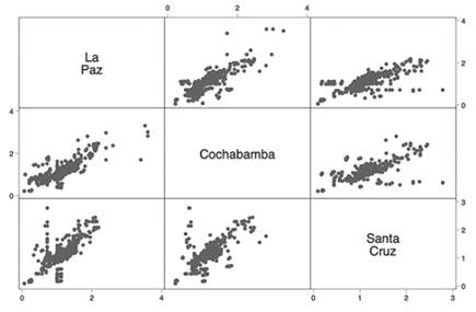
Source: Author’s calculation based on scanner transaction data at the product level from major supermarket chains.
Figure 8: Price Association Across Stores by City. January 2024 to January 2025
Notes: The figure plots level.
Estimates of the Elasticity of Substitution
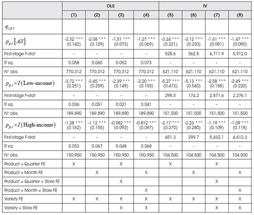
Table 2 presents estimates of the elasticity of substitution obtained by regressing monthly purchased quantities on consumer prices for all product varieties (including continuing, entering, or exiting varieties) for all periods (from January 2024 to January 2025) Panel (a) present the estimates for the full sample, Panel (b) for the low-income group, and Panel (c) for the high-income group. Columns (1) to (4) present the Ordinary Least Squares (OLS) estimates. Columns (5) to (8) present the Instrumental Variable (IV) estimates. Each column presents different specifications, allowing fixed effects to vary at the product and store levels, while filtering out income-specific price indices and variety-level demand shifters. Notice that elasticities are negative and statistically significant under all specifications and remain below the theoretical limit of -1. IV estimates are statistically efficient and clustered at the store- product level. Furthermore, our instrument appears robust, as indicated by a significant first- stage F-statistic across all specifications and income groups, suggesting that supermarkets use near-uniform pricing.
At the aggregate level, OLS elasticities vary from -2.32 using the product-quarter fixed effects in column (1) to -2.08 using the more detailed product-month fixed effects in column (2). Allowing demand shifters and price indices to differ across locations, in columns (3) and (4), resulted in estimated elasticities of -1.53 and -1.27, respectively. IV estimates, reported in columns (5)-(8), indicate more elastic demand curves than the OLS counterparts. In our basic setup, the IV estimates are -3.24 and -3.12 for product-quarter and product-monthly fixed effects, respectively, while the OLS estimates are -2.34 and -2.087.
By income group, high-income consumers exhibit higher substitution elasticities than low-income consumers under all specifications. In the basic setup, OLS estimates for high- income consumers are -3.72 and 3.45, while for their low-income counterparts, elasticities are -1.28 and 1.12 for product-quarter and product-monthly fixed effects, respectively. IV estimates also show more elastic demand curves than the corresponding OLS estimates. In the basic setup, IV estimates for high-income consumers are -5.27 and 5.13, while for their low-income counterparts, elasticities are -2.17 and 2.23 for product-quarter and product- monthly fixed effects, respectively.
Table 2 Estimates of the Elasticity of Substitution. Aggregate and by Income Strata
Source: Author’s calculation based on scanner transaction data at the product level from major supermarket chains from January 2024 to January 2025.
Notes: This table presents estimates of the elasticities of substitution using unweighted regressions and cluster standard errors at the category-store level. The top Panel reports aggregate estimates across all income groups. The medium and bottom panels report estimates for low-income and high-income consumers. Columns (1)-(4) display ordinary least squares (OLS) estimates; columns (5)-(8) present instrumental variable (IV) estimates. The first-stage F-statistic referenced is the effective first-stage F-statistic (Montiel-Olea and Pflueger, 2013). Standard errors are reported in parentheses below the coefficient. Significance levels are indicated as follows: 10% (*), 5% (**), and 1% (***).
In summary, our results present clear evidence that high-income consumers exhibit higher substitution elasticities than low-income consumers, suggesting that high-income consumers view alternatives in their choice set as more substitutable and place a higher value on product variety changes than their low-income counterparts. This is a finding that has been consistently observed in the related literature8.
Cost of Living Effects
Aggregate Effects
Figure 9 reports the decomposition of the total cost of living effects of devaluation for all consumers into four components: changes in marginal cost, retail margins, substitution across products, and product variety. The cost of living rose steadily during the period of analysis to 13% after one year. The primary driver of this increase was the increasing marginal costs of ongoing product varieties. The marginal cost of food and beverages increased by almost 17%, corresponding to an aggregate pass-through rate into marginal costs of 21%, which is lower than the range of estimates provided by the literature (Gopinath et al., 2020)9. The cost-of-living effect is lower than the marginal cost increase due to compensatory changes in retail markups, substitution, and the availability of different varieties. Consistent with profit- maximizing behavior, firms reduced their markup by 1%. Substitution of more expensive products by cheaper products in the same category reduces the cost of living by 1.5%. Finally, changes in the availability of varieties reduced the increase in the cost of living by about 2.5%, suggesting that the taste-based price of newly introduced varieties was more favorable than those that exited the market.
Source: Author’s calculation based on scanner transaction data at the product level from major supermarket chains.
Figure 9: Decomposition of the Cost of Living Effects of devaluation, January 2024 to January 2025. Full Sample
Notes: The figure decomposes the change in the cost of living into a price channel that includes (i) a marginal cost channel, (ii) a markup channel, (iii) a substitution channel, and (iv) a product variety channel.
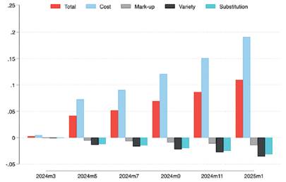
Effects by Income Strata
To assess the distributional impacts, Figure 10 reports the decomposition of the cost of living for low-income (panel a) and high-income consumers (panel b). We find that high-income consumers have lower cost-of-living increases than low-income consumers despite higher increases in the marginal cost of their basket of goods. While the marginal cost increases by 14.6% for the high-income consumers, their cost of living increases only by 10.9% because markup, variety, and substitution channels counterbalance part of the changes in marginal cost. This aligns with the observation that high-income consumers generally have a higher expenditure share on premium foreign varieties, whose costs increased more significantly. To maximize profit, supermarkets have absorbed part of the increase in marginal cost and reduced retail markups by 1.4% after devaluation. Furthermore, since high-income consumers have lower elasticities of substitution, they also substitute away from expensive varieties by 3.1% and benefit more from changes in product variety that occurred after devaluation by 3.5%.
On the other hand, low-income consumers, who face a 14.6% increase in marginal cost in their basket of goods, face an increase in their cost of living of 13.4%. Because low-income consumers’ spending on foreign varieties goes to necessities rather than luxuries, and they have lower elasticities of substitution, they are forced to absorb almost all increases in the marginal costs. Jointly, the markup, substitution, and variety channels offset only -0.01% of the marginal cost increase.
Our results shed light on the importance of examining markups, varieties, and substitution channel changes when analyzing the transmission mechanisms of exchange rate shocks to consumer prices. In particular, our results highlight the role that the elasticity of substitution plays not only across products and varieties but also for markup movements that can offset the relative price adjustment after a devaluation. Furthermore, we show that differences in the increase in marginal cost between high- and low-income consumers can be reversed by markups, varieties, and substitution channels, producing substantial cost-of-living inequalities between the poor and the rich. These differences in the cost-of-living increase between the rich and the poor give us a glimpse of the direction of the distributional effects of the devaluation.
Source: Author’s calculation based on scanner transaction data at the product level from major supermarket chains.
Figure 10: Decomposition of the Cost of Living Effects of Devaluation, January 2024 to January 2025. By Income Strata
Notes: The figure decomposes the change in the cost of living into a price channel that includes (i) a marginal cost channel, (ii) a markup channel, (iii) a substitution channel, and (iv) a product variety channel.
Table 3 Decomposing Total Cost of Living Effects. By Income Strata. January 2024 to January 2025
Source: Author’s calculation based on scanner transaction data at the product level from major supermarket chains.
Notes: The figure decomposes the change in the cost of living into a price channel that includes (i) a marginal cost channel, (ii) a markup channel, (iii) a substitution channel, and (iv) a product variety channel.
Distributional Consequences
The cost-of-living effects estimate the devaluation’s welfare cost on food and beverages expenditure, not total outlays. While food is the largest expenditure category for lower‐income households, other expenditure categories are likely to be affected by devaluation, including spending on prepared food (the larger share of the hospitality category) and clothing.
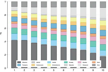
Figure 11 reports the budget share by expenditure category across per capita income deciles based on the Household Budget Survey from 2019. As Engel’s law predicts, they devote a larger fraction of their budgets to food and beverages (more than 40% for the first decile). Food budget shares reach and shrink steadily to 20% for the richest decile. By contrast, in the upper deciles, we see larger slices for more discretionary spending categories such as hospitality and entertainment, and investments in education, health, and durable goods. These slices are relatively small among poorer households but expand as incomes increase. Notably, housing expenditures do not grow nearly as much as discretionary categories. Transport and Communication also shih moderately, often accounting for a slightly more significant share in the middle deciles.
Source: Author’s calculation based on Household Budget Survey 2019.
Figure 11: Budget Share of Expenditure Categories by Decile of Per Capita Household Income
Notes: The figure shows the budget share of different expenditure categories by decile of per capita household income. Each vertical bar corresponds to a particular decile (from 1 to 10 along the horizontal axis), and the stacked sections within each bar indicate the share of total expenditure devoted to a specific expenditure category within that decile. Expenditure categories include Food and Beverages, Alcohol and Tobacco, Transport, Communication and Clothing, Housing, Durables and Furniture, Health, Entertainment, Education, Hospitality, and other expenses.
To estimate the devaluation total welfare effect, not only the impact on food expenditure but on total expenditure, we can use the most recent available Household survey (2023) “nowcasted” to the year 202410, and simulate a series of scenarios that extrapolate our cost of living estimates to different per capita income deciles and expenditure categories. We explore three different scenarios: Scenario 1 applies the high-income effect to the first quantile and the low-income impact to the remaining households, only for food expenditures, without considering devaluation effects on other expenditure categories. Scenario 2 applies the high- income effect to the first quantile, the low-income impact on the food expenditures of the remaining households, and the high-income effect on prepared food expenditures. Scenario 3 applies the high-income effect to the first quantile, the low-income impact on the rest of the households in terms of food expenditures, and the high-income impact on spending for prepared food and clothing.
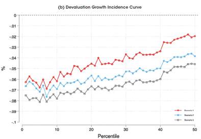
Figure 12 presents the distributional effects of devaluation for all three scenarios. Panel A presents the changes in the cumulative per capita income distribution, i.e., how many more or fewer people are at every percentile of the income distribution. Panel B presents the devaluation growth incidence curve (GIC), i.e., the growth in per capita income welfare by percentile. The devaluation’s impact on the GIC appears regressive, with households in the lower income distribution suffering greater welfare reductions than those in the upper part.
Source: Author’s calculation based on estimated cost of living effects by income strata.
Figure 12: Distributional Effects of the Currency Crisis, by Income Percentile. January 2024 to January 2025
Notes: The figure applies the cost-of-living effect only to the food budget share. We present three scenarios. Scenario 1 applies the high-income effect to the first quantile and the low-income effect to the rest of the households, only to food expenditures, without considering devaluation effects on other expenditure categories. Scenario 2 applies the high-income effect to the first quantile, the low-income impact on the food expenditures of the remaining households, and the high-income effect on prepared food expenditures. Scenario 3 applies the high-income effect to the first quantile, the low-income impact on the rest of the households in terms of food expenditures, and the high-income impact on expenditures for prepared food and clothing. Panel (a) presents the changes in the cumulative per capita income distribution, i.e., how many more (or fewer) fraction of people are at every percentile of the income distribution. Panel (b) presents the devaluation growth incidence curve (GIC), i.e., the per capita income welfare growth (loss) by percentile.
Poverty and Inequality Effects
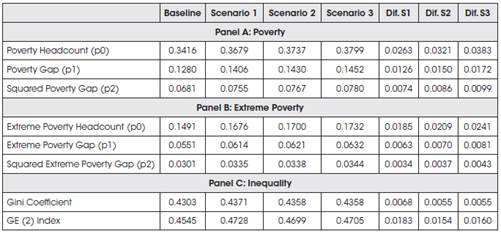
Table 4 presents the devaluation effects on poverty and inequality through prices for the three scenarios. Bolivia’s de facto currency devaluation over the last year has increased the poverty headcount by 2.6 and 3.8 percentage points and the poverty gap (the average distance of the poor from the poverty line) by 1.3 and 1.7 percentage points. In terms of extreme poverty, i.e., being unable to cover basic food expenditures, we find that last year’s devaluation is associated with a 1.8 to 2.4 percentage point increase in the headcount and a 0.6 to 0.8 percentage point increase in the poverty gap. Finally, devaluation is associated with increased inequality, ranging from 0.7 to 0.5 points in the Gini index and 1.8 to 1.6 in the Atkinson index. The induced increase in poverty and income inequality is associated with the larger erosion of purchasing power that affects the bottom deciles. Poorer households spend a large share of their budget on foreign necessities, and they have fewer possibilities to substitute them. They are forced to absorb almost all increases in marginal cost, with few options to substitute essentials (e.g., wheat-based products, beans, pasta). Households near the poverty line may fall below it due to these pressures, especially if labor earnings do not adjust to compensate for higher living costs. On the other hand, higher-income households can adjust their consumption patterns more easily and substitute luxury and premium foreign items (e.g., chocolates, spices, coffee) for cheaper or new varieties than lower-income groups. Significant differential impacts in cost- of-living increases can lead to poverty and worsen economic inequality.
A devaluation affects household welfare through multiple channels. The price pass-through of devaluation leads to higher prices for both foreign and local varieties (due to increased input costs). While the pass-through effect is greater for foreign varieties consumed by high- income households, the distributional impact disproportionately affects low-income people. This occurs because the increasing marginal cost faced by low-income families is not offset by reductions in retail markup or substitution effects, which higher-income households can take advantage of. Consequently, poorer households bear almost all of the increase in marginal costs without the advantage of retail margin adjustments or substitution opportunities.
Table 4 Poverty and Inequality Consequences of Devaluation
Source: Author’s calculation based on estimated cost of living effects by income strata.
Notes: The figure applies the cost-of-living effect only to the food budget share. We use the effect of high- income consumers for the top 20% and the effect of low-income consumers for the rest of the quintiles.
Limitations
Tracking prices using scanner data allows us to assess inflation pass-through and its impacts on the cost of living and household welfare more granularly and in real-time. Still, it does not account for employment dynamics and wage adjustments. Our analysis of devaluation effects only accounts for the welfare effects generated by price dynamics. It does not account for the potential impact of devaluation on employment and labor earnings. If devaluation boosts exports, we might observe employment and wage increases in some tradable sectors. At the same time, we may also observe a reduction in profits and employment incentives in small or medium-sized businesses that trade imported goods due to lower demand and higher prices for imports.
Despite these limitations, the data-driven approach employed in this study offers significant advantages over Computational General Equilibrium (CGE) models. While CGE models provide a theoretically consistent macroeconomic framework, they often rely on strong assumptions regarding functional forms, perfect competition, and rational agent behavior. They require extensive calibration and may not accurately reflect the structure of economies with large informal sectors, as is the case in Bolivia. This hinders their usefulness in analyzing differential impacts for different populations. Although valuable for policy simulations, CGE models may overlook short-term distributional effects and consumer adaptation strategies that are more accurately captured in transaction-level data. By focusing on observed price and consumption behavior rather than theoretical equilibrium conditions, this study provides a more grounded empirical basis for understanding the immediate and tangible effects of devaluation on different income groups.
Conclusions
This paper uses scanner transaction data, at the product level, from a major supermarket chain to analyze the price and welfare dynamics during the Bolivia currency crisis - the period spanning from January 2024 to January 2025, where we observe a de facto devaluation of the boliviano of more than 60% in the black market. While expenditure in a formal supermarket leaves out informal market dynamics, we show that, at least in terms of price changes, price changes at the supermarket level correspond to observed price changes in the overall consumer price index for most products and at the subcategory level for the food and beverage category.
First, we estimate the pass-through effects of devaluation on consumer prices (% after a year) and highlight the asymmetric impact of devaluation on foreign (16%) and local varieties (9%), likely due to increases in input prices. We also report the asymmetric effect on high- income consumers (18%) and low-income consumers (14%). This modest pass-through effect of a 60% de facto devaluation might be explained by a combination of fuel and food subsidies and price controls that help maintain affordable prices for key items in the food basket, such as bread. For example, indirect subsidies exceeding 50% for wheat flour have helped keep the prices of bread and other wheat-based products relatively stable. Additionally, export restrictions on oil and bread contributed to the relatively low pass-through effect of the devaluation.
Second, we assume a nested CES structure of preferences and estimate elasticities of substitution for the full sample, as well as for high- and low-income consumers. We use these estimates to decompose the total price effect into a price channel that groups change in marginal cost and retail margins, a substitution channel, and a product variety channel. Our analysis reveals significant differences in how price increases affect the cost of living of low and high-income consumers. For low-income consumers, the cost-of-living increase of 13.5% after one year can be explained mainly by rising costs for both local and foreign varieties, which were fully passed on to them, with no substantial changes in markup and no significant substitution or variety effects. In contrast, high-income consumers had a lower annual increase in their cost of living (10.9%) because, despite facing higher marginal cost increases (19.1%), this increase was offset by a decrease in markups of 1.5%, a substitution effect of -3.1% and a variety effect of -3.1%. Because high-income consumers’ baskets of foreign goods include luxury and premium items (such as spices, chocolates, coffee, and seasonal fruits), and they have higher elasticities of substitution following a currency crisis devaluation, they can protect themselves from price increases by substituting away from foreign varieties toward cheaper local varieties. Furthermore, because they can avoid expensive imports, sellers increase their varieties and reduce their retail markups to keep part of the demand, further protecting high- income consumers. On the other hand, since low-income consumers’ baskets of foreign goods mainly include essential imported goods such as staples and other necessities, their elasticities of substitution are much lower. This means they can fully absorb the marginal cost increase with negligible compensatory effects from changes in retail margins, substitution, or variety.
Finally, we analyze the potential distributional consequences of food and beverage expenditures and total per capita expenditures and calculate the implied changes in the per capita income distribution, summarized by a devaluation negative and regressive growth incidence curve, as well as implied changes in poverty and inequality indicators. Depending on the different assumptions about the cost-of-living effects on non-food expenditures, such as prepared food (hospitality), clothing, and other non-food items, we find that devaluation has significant regressive consequences for income distribution. Because they allocate a larger share of their budget to food, devaluation reduces the total welfare of the poorest between 6 and 8%. In comparison, it only reduces the total welfare of the richest between 2 and 5% since they allocate a smaller share of their budget to food. The disproportionate welfare losses of low- income households increase poverty (incidence and the gap) and increase overall inequality (as measured by different inequality indicators). It is crucial to note that our analysis is a lower bound, as it does not account for welfare changes that occur in some inelastic products, such as medicines and auto parts, which have limited substitutes. Another limitation of the study is that it does not account for employment dynamics and wage adjustments.
Policy Implications: What’s Next for Bolivia?
The persistence of macroeconomic imbalances and the significant discrepancies between official and black market exchange rates highlight the urgent need for structural adjustment policies. These policies should prevent further distortions and guide the country away from economic instability. While the official peg is unsustainable, a formal devaluation needs to be accompanied, not only by sound macroeconomic policies, that improve economic stability and restore a more predictable policy environment but also by effective welfare programs, that help the poor offset the adjustment impacts on their cost of living and welfare. This paper presents clear evidence that the welfare effects of a devaluation on the poor, at least in the short term, are disproportionately large and can be very painful. Therefore, carefully designed programs are needed that protect the purchasing power of the poor and prevent them from having to sell or compromise their already limited productive assets to finance the consumption of their necessities.
Bolivia has long relied on fuel subsidies (for gasoline, diesel, and natural gas) and basic food subsidies, particularly for wheat flour, as cornerstones of its price stabilization policies. While universal subsidies protect consumers from price shocks and ensure access to staple foods, they also present complex challenges, including (1) high fiscal costs, (2) market distortions, and (3) unintended redistributive consequences. Since universal subsidies cannot exclude affluent households, they tend to be regressive in nature. Middle- and high-income urban and peri-urban families receive a larger share of the subsidy, while the poorest families in rural areas benefit less, resulting in regressive distributional effects. We need to consider new policies, including well-targeted compensatory cash transfers and food vouchers, that allow us to phase out universal subsidies in favor of more effective policies. This will help avoid the scars from necessary macroeconomic adjustments and alleviate the growing frustration of the poor.